Using Double Machine Learning and Linear Programming to optimise treatment strategies

Causal AI, exploring the integration of causal reasoning into machine learning

What is this series of articles about?

Welcome to my series on Causal AI, where we will explore the integration of causal reasoning into machine learning models. Expect to explore a number of practical applications across different business contexts.

In the last article we explored de-biasing treatment effects with Double Machine Learning. This time we will delve further into the potential of DML covering using Double Machine Learning and Linear Programming to optimise treatment strategies.

If you missed the last article on Double Machine Learning, check it out here:

De-biasing Treatment Effects with Double Machine Learning

Introduction

This article will showcase how Double Machine Learning and Linear Programming can be used optimise treatment strategies:

Expect to gain a broad understanding of:

• Why businesses want to optimise treatment strategies.
• How conditional average treatment effects (CATE) can help personalise treatment strategies (also known as Uplift modelling).
• How Linear Programming can be used to optimise treatment assignment given budget constraints.
• A worked case study in Python illustrating how we can use Double Machine Learning to estimate CATE and Linear Programming to optimise treatment strategies.

The full notebook can be found here:

causal_ai/notebooks/estimating average treatment effects with double machine learning.ipynb at main · raz1470/causal_ai

Optimising treatment strategies

There is a common question which arises in most businesses: “What is the optimal treatment for a customer in order to maximise future sales whilst minimising cost?”.

Let’s break this idea down with a simple example.

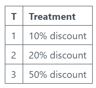
Your business sells socks online. You don’t sell an essential product, so you need to encourage existing customers to repeat purchase. Your main lever for this is sending out discounts. So the treatment strategy in this case is sending out discounts:

• 10% discount
• 20% discount
• 50% discount

Each discount has a different return on investment. If you think back to the last article on average treatment effects, you can probably see how we can calculate ATE for each of these discounts and then select the one with the highest return.

However, what if we have heterogenous treatment effects — The treatment effect varies across different subgroups of the population.

This is when we need to start considering conditional average treatment effects (CATE)!

Conditional Average Treatment Effects (CATE)

CATE

CATE is the average impact of a treatment or intervention on different subgroups of a population. ATE was very much about “does this treatment work?” whereas CATE allows us to change the question to “who should we treat?”.

We “condition” on our control features to allow treatment effects to vary depending on customer characteristics.

Think back to the example where we are sending out discounts. If customers with a higher number of previous orders respond better to discounts, we can condition on this customer characteristic.

It is worth pointing out that in Marketing, estimating CATE is often referred to as Uplift Modelling.

Estimating CATE with Double Machine Learning

We covered DML in the last article, but just in case you need a bit of a refresher:

“First stage:

• Treatment model (de-biasing): Machine learning model used to estimate the probability of treatment assignment (often referred to as propensity score). The treatment model residuals are then calculated.
• Outcome model (de-noising): Machine learning model used to estimate the outcome using just the control features. The outcome model residuals are then calculated.

Second stage:

• The treatment model residuals are used to predict the outcome model residuals.”

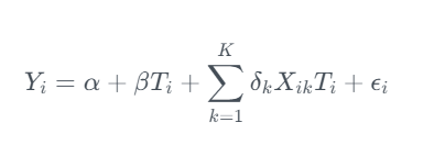
We can use Double Machine Learning to estimate CATE by interacting our control features (X) with the treatment effect in the second stage model.

This can be really powerful as we are now able to get customer level treatment effects!

Linear Programming

What is it?

Linear programming is an optimisation method which can be used to find the optimal solution of a linear function given some constraints. It is often used to solve transportation, scheduling and resource allocation problems. A more generic term which you might see used is Operations Research.

Let’s break linear programming down with a simple example:

• Decision variables: These are the unknown quantities which we want to estimate optimal values for — The marketing spend on Social Media, TV and Paid Search.
• Objectives function: The linear equation we are trying to minimise or maximise — The marketing Return on Investment (ROI).
• Constraints: Some restrictions on the decision variables, usually represented by linear inequalities — Total marketing spend between £100,000 and £500,000.

The intersection of all constraints forms a feasible region, which is the set of all possible solutions that satisfy the given constraints. The goal of linear programming is to find the point within the feasible region that optimizes the objective function.

Assignment problems

Assignment problems are a specific type of linear programming problem where the goal is to assign a set of “tasks” to a set of “agents”. Lets use an example to bring it to life:

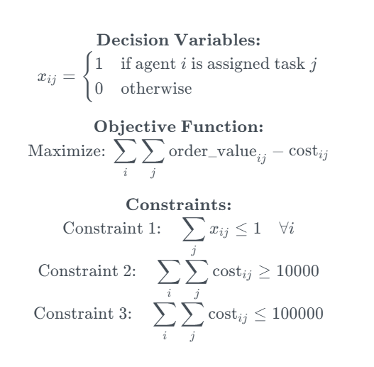
You run an experiment where you send different discounts out to 4 random groups of existing customers (the 4th of which actually you don’t send any discount). You build 2 CATE models — (1) Estimating how the offer value effects the order value and (2) Estimating how offer value effects the cost.

• Agents: Your existing customer base
• Tasks: Whether you send them a 10%, 20% or 50% discount
• Decision variables: Binary decision variable
• Objective function: The total order value minus costs
• Constraint 1: Each agent is assigned to at most 1 task
• Constraint 2: The cost ≥ £10,000
• Constraint 3: The cost ≤ £100,000

We basically want to find out the optimal treatment for each customer given some overall cost constraints. And linear programming can help us do this!

It is worth noting that this problem is “NP hard”, a classification of problems that are at least as hard as the hardest problems in NP (nondeterministic polynomial time).

Linear programming is a really tricky but rewarding topic. I’ve tried to introduce the idea to get us started — If you want to learn more I recommend this resource:

Hands-On Linear Programming: Optimization With Python – Real Python

OR Tools

OR tools is an open source package developed by Google which can solve a range of linear programming problems, including assignment problems. We will demonstrate it in action later in the article.

OR-Tools | Google for Developers

Marketing Case Study

Background

We are going to continue with the assignment problem example and illustrate how we can solve this in Python.

Data generating process

We set up a data generating process with the following characteristics:

• Difficult nuisance parameters (b)
• Treatment effect heterogeneity (tau)

The X features are customer characteristics taken before the treatment:

T is a binary flag indicating whether the customer received the offer. We create three different treatment interactions to allow us to simulate different treatment effects.

def data_generator(tau_weight, interaction_num):
    
    # Set number of observations
    n=10000

    # Set number of features
    p=10

    # Create features
    X = np.random.uniform(size=n * p).reshape((n, -1))

    # Nuisance parameters
    b = (
        np.sin(np.pi * X[:, 0] * X[:, 1])
        + 2 * (X[:, 2] - 0.5) ** 2
        + X[:, 3]
        + 0.5 * X[:, 4]
        + X[:, 5] * X[:, 6]
        + X[:, 7] ** 3
        + np.sin(np.pi * X[:, 8] * X[:, 9])
    )

    # Create binary treatment
    T = np.random.binomial(1, expit(b))

    # treatment interactions
    interaction_1 = X[:, 0] * X[:, 1] + X[:, 2]
    interaction_2 = X[:, 3] * X[:, 4] + X[:, 5]
    interaction_3 = X[:, 6] * X[:, 7] + X[:, 9]

    # Set treatment effect
    if interaction_num==1:
        tau = tau_weight * interaction_1
    elif interaction_num==2:
        tau = tau_weight * interaction_2
    elif interaction_num==3:
        tau = tau_weight * interaction_3

    # Calculate outcome
    y = b + T * tau + np.random.normal(size=n)
    
    return X, T, tau, y

We can use the data generator to simulate three treatments, each with a different treatment effect.

np.random.seed(123)

# Generate samples for 3 different treatments
X1, T1, tau1, y1 = data_generator(0.75, 1)
X2, T2, tau2, y2 = data_generator(0.50, 2)
X3, T3, tau3, y3 = data_generator(0.90, 3)

As in the last article, the data generating process python code is based on the synthetic data creator from Ubers Causal ML package:

causalml/causalml/dataset/regression.py at master · uber/causalml

Estimating CATE with DML

We then train three DML models using LightGBM as flexible first stage models. This should allow us to capture the difficult nuisance parameters whilst correctly calculating the treatment effect.

Pay attention to how we pass the X features in through X rather than W (unlike in the last article where we passed the X features through W). Features passed through X will be used in both the first and second stage models — In the second stage model the features are used to create interaction terms with the treatment residual.

np.random.seed(123)

# Train DML model using flexible stage 1 models
dml1 = LinearDML(model_y=LGBMRegressor(), model_t=LGBMClassifier(), discrete_treatment=True)
dml1.fit(y1, T=T1, X=X1, W=None)

# Train DML model using flexible stage 1 models
dml2 = LinearDML(model_y=LGBMRegressor(), model_t=LGBMClassifier(), discrete_treatment=True)
dml2.fit(y2, T=T2, X=X2, W=None)

# Train DML model using flexible stage 1 models
dml3 = LinearDML(model_y=LGBMRegressor(), model_t=LGBMClassifier(), discrete_treatment=True)
dml3.fit(y3, T=T3, X=X3, W=None)

When we plot the actual vs estimated CATE, we see that the model does a reasonable job.

# Create a figure and subplots
fig, axes = plt.subplots(1, 3, figsize=(15, 5))

# Plot scatter plots on each subplot
sns.scatterplot(x=dml1.effect(X1), y=tau1, ax=axes[0])
axes[0].set_title('Treatment 1')
axes[0].set_xlabel('Estimated CATE')
axes[0].set_ylabel('Actual CATE')

sns.scatterplot(x=dml2.effect(X2), y=tau2, ax=axes[1])
axes[1].set_title('Treatment 2')
axes[1].set_xlabel('Estimated CATE')
axes[1].set_ylabel('Actual CATE')

sns.scatterplot(x=dml3.effect(X3), y=tau3, ax=axes[2])
axes[2].set_title('Treatment 3')
axes[2].set_xlabel('Estimated CATE')
axes[2].set_ylabel('Actual CATE')

# Add labels to the entire figure
fig.suptitle('Actual vs Estimated')

# Show plots
plt.show()

Naive optimisation

We will start by exploring this as an optimisation problem. We have a three treatments which a customer could receive. Below we create a mapping for the cost of each treatment, and set an overall cost constraint.

# Create mapping for cost of each treatment
cost_dict = {'T1': 0.1, 'T2': 0.2, 'T3': 0.3}

# Set constraints
max_cost = 3000

We can then estimate the CATE for each customer and then initially select each customers best treatment. However, selecting the best treatment doesn’t keep us within the maximum cost constraint. Therefore select the customers with the highest CATE until we reach our max cost constraint.

# Concatenate features
X = np.concatenate((X1, X2, X3), axis=0)

# Estimate CATE for each treatment using DML models
Treatment_1 = dml1.effect(X)
Treatment_2 = dml2.effect(X)
Treatment_3 = dml3.effect(X)
cate = pd.DataFrame({"T1": Treatment_1, "T2": Treatment_2, "T3": Treatment_3})

# Select the best treatment for each customer
best_treatment = cate.idxmax(axis=1)
best_value = cate.max(axis=1)

# Map cost for each treatment
best_cost = pd.Series([cost_dict[value] for value in best_treatment])

# Create dataframe with each customers best treatment and associated cost
best_df = pd.concat([best_value, best_cost], axis=1)
best_df.columns = ["value", "cost"]
best_df = best_df.sort_values(by=['value'], ascending=False).reset_index(drop=True)

# Naive optimisation
best_df_cum = best_df.cumsum()
opt_index = best_df_cum['cost'].searchsorted(max_cost)
naive_order_value = round(best_df_cum.iloc[opt_index]['value'], 0)
naive_cost_check = round(best_df_cum.iloc[opt_index]['cost'], 0)

print(f'The total order value from the naive treatment strategy is {naive_order_value} with a cost of {naive_cost_check}')

Optimising treatment strategies with Linear Programming

We start by creating a dataframe with the cost of each treatment for each customer.

# Cost mapping for all treatments
cost_mapping = {'T1': [cost_dict["T1"]] * 30000,
                'T2': [cost_dict["T2"]] * 30000,
                'T3': [cost_dict["T3"]] * 30000}

# Create DataFrame
df_costs = pd.DataFrame(cost_mapping)

Now it’s time to use the OR Tools package to solve this assignment problem! The code takes the following inputs:

• Cost constraints
• Array containing the cost of each treatment for each customer
• Array containing the estimated order value for each treatment for each customer

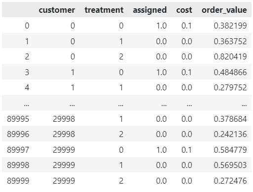
The code outputs a dataframe with each customers potential treatment, and a column indicating which one is the optimal assignment.

solver = pywraplp.Solver.CreateSolver('SCIP')

# Set constraints
max_cost = 3000
min_cost = 3000

# Create input arrays
costs = df_costs.to_numpy()
order_value = cate.to_numpy()

num_custs = len(costs)
num_treatments = len(costs[0])

# x[i, j] is an array of 0-1 variables, which will be 1 if customer i is assigned to treatment j.
x = {}
for i in range(num_custs):
    for j in range(num_treatments):
        x[i, j] = solver.IntVar(0, 1, '')
    
# Each customer is assigned to at most 1 treatment.
for i in range(num_custs):
    solver.Add(solver.Sum([x[i, j] for j in range(num_treatments)]) <= 1)

# Cost constraints
solver.Add(sum([costs[i][j] * x[i, j] for j in range(num_treatments) for i in range(num_custs)]) <= max_cost)
solver.Add(sum([costs[i][j] * x[i, j] for j in range(num_treatments) for i in range(num_custs)]) >= min_cost)

# Objective
objective_terms = []
for i in range(num_custs):
    for j in range(num_treatments):
        objective_terms.append((order_value[i][j] * x[i, j] - costs[i][j] * x[i, j] ))
solver.Maximize(solver.Sum(objective_terms))

# Solve
status = solver.Solve()

assignments = []
values = []

if status == pywraplp.Solver.OPTIMAL or status == pywraplp.Solver.FEASIBLE:
    for i in range(num_custs):
        for j in range(num_treatments):
            # Test if x[i,j] is 1 (with tolerance for floating point arithmetic).
            if x[i, j].solution_value() > -0.5:
                assignments.append([i, j])
                values.append([x[i, j].solution_value(), costs[i][j] * x[i, j].solution_value(), order_value[i][j]])

# Create a DataFrame from the collected data
df = pd.DataFrame(assignments, columns=['customer', 'treatment'])
df['assigned'] = [x[0] for x in values]
df['cost'] = [x[1] for x in values]
df['order_value'] = [x[2] for x in values]

df

Whilst keeping to the cost constraint of £3k, we can generate £18k in order value using the optimised treatment strategy. This is 36% higher than the naive approach!

opt_order_value = round(df['order_value'][df['assigned'] == 1].sum(), 0)
opt_cost_check = round(df['cost'][df['assigned'] == 1].sum(), 0)

print(f'The total order value from the optimised treatment strategy is {opt_order_value} with a cost of {opt_cost_check}')

Final thoughts

Today we covered using Double Machine Learning and Linear Programming to optimise treatment strategies. Here are some closing thoughts:

• We covered Linear DML, you may want to explore alternative approaches which are more suited to dealing with complex interaction effects in the second stage model:

EconML/notebooks/Double Machine Learning Examples.ipynb at main · py-why/EconML

• But also remember you don’t have to use DML, other methods like T-Learner or DR-Learner could be used.
• To keep this article to a quick read I did not tune the hyper-parameters — As we increase the complexity of the problem and approach used, we need to pay closer attention to this part.
• Linear programming/assignment problems are NP hard, so if you have a large customer base and/or several treatments this part of the code may take a long time to run.
• It can be challenging operationalising a daily pipeline with linear programming/assignment problems — An alternative is running the optimisation periodically and learning the optimal policy based on the results in order to create a segmentation to use in a daily pipeline.

Follow me if you want to continue this journey into Causal AI — In the next article we will explore how we can estimate non-linear treatment effects in pricing and marketing optimisation problems.

Using Double Machine Learning and Linear Programming to optimise treatment strategies was originally published in Towards Data Science on Medium, where people are continuing the conversation by highlighting and responding to this story.