Unit Disk Uniform Sampling

Discover the optimal transformations to apply on the standard [0,1] uniform random generator for uniformly sampling a 2D disk

0. Introduction

In my previous article on Unit Disk and 2D Bounded KDE, I discussed the importance of being able to sample arbitrary distributions. This is especially relevant for applications like Monte Carlo integration, which is used to solve complex integrals, such as light scattering in Physically Based Rendering (PBRT).

Sampling in 2D introduces new challenges compared to 1D. This article focuses on uniformly sampling the 2D unit disk and visualizing how transformations applied to a standard [0,1] uniform random generator create different distributions.

We’ll also explore how these transformations, though yielding the same distribution, affect Monte Carlo integration by introducing distortion, leading to increased variance.

1. How to sample a disk uniformly?

Introduction

Random number generators often offer many predefined sampling distributions. However, for highly specific distributions, you’ll likely need to create your own. This involves combining and transforming basic distributions to achieve the desired outcome.

For instance, to uniformly sample the interval between a and b, you can apply an affine transform on the standard uniform sampling from [0,1].

In this article, we’ll explore how to uniformly sample points within the 2D unit disk by building on the basic [0,1] uniform sampling.

For readability, I’ve intentionally used the adjective “unit” in two different contexts in this article. The “unit square” refers to the [0,1]² domain, reflecting the range of the basic random generator. Conversely, the “unit disk” is described within [-1,1]² for convenience in polar coordinates. In practice, we can easily map between these using an affine transformation. We’ll denote u and v as samples drawn from the standard [0,1] or [-1,1] uniform distribution.

Rejection Sampling

Using the [0,1] uniform sampling twice allows us to uniformly sample the unit square [0,1]².

A very simple approach known as “Rejection Sampling” consists in sampling the unit square and rejecting any sample falling outside the disk.

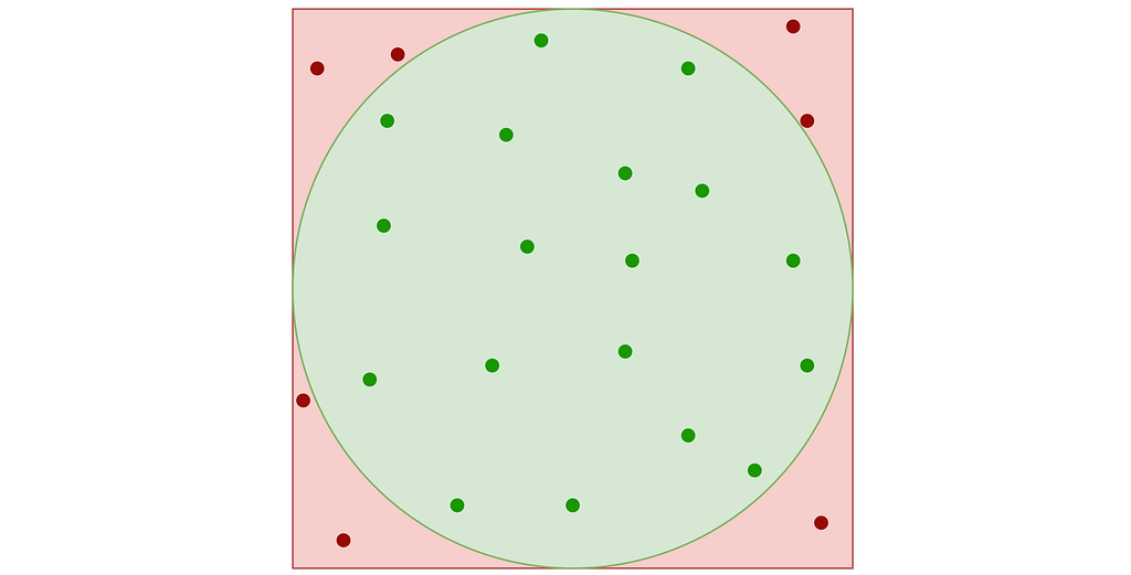
This results in points that follow a uniform 2D distribution within the disk contained in the unit square, as illustrated in the figure below.

The density maps in this article are generated by sampling many points from the specified distribution and then applying a Kernel Density Estimator. Methods for addressing boundary bias in the density are detailed in the previous article “Unit Disk and 2D Bounded KDE”.

A major drawback is that rejection sampling can require many points to get the desired number of valid samples, with no upper limit on the total number, leading to inefficiencies and higher computational costs.

Intuitive Polar Sampling

An intuitive approach is to use polar coordinates for uniform sampling: draw a radius within [0,1] and an angle within [0, 2π].

Both the radius and angle are uniform, what could possibly go wrong?However, this method leads to an infinite density singularity at the origin, as illustrated by the empirical density map below.

To ensure the linear colormap remains readable, the density map has been capped at an arbitrary maximum value of 10. Without this cap, the map would display a single red dot at the center of a blue disk.

The figure below uses color to show how the unit square, sampled with (u,v), maps to the unit disk with (x,y) using the polar transform defined above. The colored areas in the square are equal, but this equality does not hold once mapped to the disk. This visually illustrates the density map: large radii exhibit much lower density, as they are distributed across a wider ring farther from the origin.

Let’s explore the mathematical details. When applying a transform T to a multi-dimensional random variable A, the resulting density is found by dividing by the absolute value of the determinant of the Jacobian of T.

The polar transform is given by the equation below.

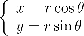
We can compute the determinant of its jacobian.

Thus, the polar transformation results in a density that is inversely proportional to the radius, explaining the observed singularity.

The 1D density profile along the diagonal shown above corresponds to the absolute value of the inverse function, which is then set to zero outside [-1, 1]. At first glance, this might seem counterintuitive, given that the 1D inverse function isn’t integrable over [-1, 1]! However, it’s essential to remember that the integration is performed in 2D using polar coordinates, not in 1D.

Uniform Polar Sampling — Differential Equation

There are two ways to find the correct polar transform that results in an uniform distribution. Either by solving a differential equation or by using the inversion method. Let’s explore both approaches.

To address the heterogeneity in the radius, we introduce a function f to adjust it: r=f(u). The angle, however, is kept uniform due to the symmetry of the disk. We can then solve the differential equation that ensures the determinant of the corresponding Jacobian remains constant, to keep the same density.

We get ff’=c, which has a unique solution given the boundary conditions f(0)=0 and f(1)=1. We end up with the following transform.

Uniform Polar Sampling — Inversion Method

The inversion method is easier to grasp in the discrete case. Consider three possible values A, B and C with probabilities of 60%, 10%, and 30%, respectively. As shown in the figure below, we can stack these probabilities to reach a total height of 100%. By uniformly drawing a percentage U between 0% and 100% and mapping it to the corresponding value A, B or C on the stack, we can transform a uniform sampling into our discrete non‑uniform distribution.

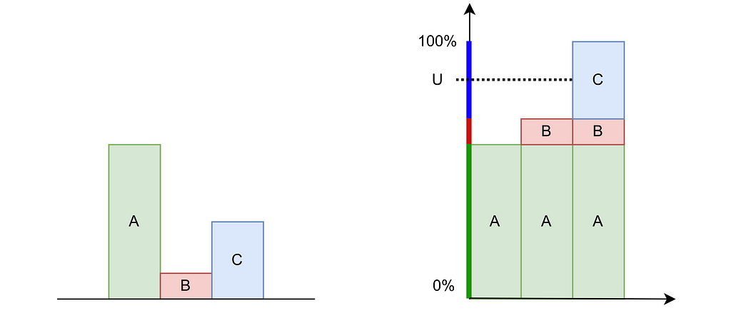
This is very similar in the continuous case. The inversion method begins by integrating the probability distribution function (PDF) p of a 1D variable X to obtain the cumulative distribution function (CDF) P(X<x), which increases from 0 to 1. Then, by sampling a uniform variable U from [0,1] and applying the inverse CDF to U, we can obtain a sample x that follows the desired distribution p.

Assuming a uniform disk distribution p(x,y), we can deduce the corresponding polar distribution p(r,θ) to enforce.

It turns out that this density p(r,θ) is separable, and we can independently sample r and θ from their respective expected 1D marginal densities using the inversion method.

When the joint density isn’t separable, we first sample a variable from its marginal density and then draw the second variable from its conditional density given the first variable.

We integrate these marginal densities into CDFs.

Sampling uniform (u,v) within [0,1] and applying the inverse CDFs gives us the following transform, which is the same as the one obtained above using the differential equation.

The resulting distribution is effectively uniform, as confirmed by the empirical density map shown below.

The square root function effectively adjusts the colored columns to preserve their relative areas when mapped to the disk.

2. How to sample a disk uniformly, but with less distortion?

Introduction

In applications like Physically Based Rendering (See PBRT (Physically Based Rendering: From Theory To Implementation), integral equations describing light scattering are solved numerically using Monte-Carlo Integration (MC).

MC Integration estimates the integral by a weighted mean of the operand evaluated at samples drawn from a given distribution. With n samples, it converges to the correct result at a rate of O(1/sqrt(n)). To halve the error, you need four times as many samples. Therefore, optimizing the sampling process to make the most of each sample is crucial.

Techniques like stratified sampling helps ensuring that all regions of the integrand are equally likely to be sampled, avoiding the redundancy of closely spaced samples that provide little additional information.

Distortion

The mapping we discussed earlier is valid as it uniformly samples the unit disk. However, it distorts areas on the disk, particularly near the outer edge. Square regions of the unit square can be mapped to very thin and stretched areas on the disk.

This distortion is problematic because the sampling on the square loses its homogeneous distribution property. Close (u,v) samples can result in widely separated points on the disk, leading to increased variance. As a result, more samples are needed in the Monte Carlo integration to offset this variance.

In this section, we’ll introduce another uniform sampling technique that reduces distortion, thereby preventing unnecessary increases in variance.

Shirley’s Concentric Mapping

In 1997, Peter Shirley published “A Low Distortion Map Between Disk and Square”. Instead of treating the uniform unit square as a plain parameter space with no spatial meaning, as we did with the radius and angle, he suggests to slightly distort the unit square into the unit disk.

The idea is to map concentric squares within the unit square into concentric circles within the unit disk, as if pinching the corners to round out the square. In the figure below, this approach appears much more natural compared to uniform polar sampling.

The unit square is divided into eight triangles, with the mapping defined for one triangle and the others inferred by symmetry.

As mentioned at the beginning of the article, it is more convenient to switch between the [0,1]² and [-1,1]² definitions of the unit square rather than using cumbersome affine transformations in the equations. Thus, we will use the [-1,1]² unit square to align with the [-1,1]² unit disk definition.

As illustrated in the figure above, the reference triangle is defined by:

Mapping the vertical edges of concentric squares to concentric arc segments means that each point at a given abscissa u is mapped to the radius r=u. Next, we need to determine the angular mapping f that results in a uniform distribution across the unit disk.

We can deduce the determinant of the corresponding Jacobian.

For a uniform disk distribution, the density within the eighth sector of the disk (corresponding to the reference triangle) is as follows.

On the other side, we have:

By combining the three previous equations and r=u , we get:

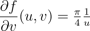
Integrating the previous equations with a zero constant to satisfy θ=0 when v=0 gives the angle mapping. Finally, we get the following mapping.

The seven others triangles are deduced by symmetry. The resulting distribution is effectively uniform, as confirmed by the empirical density map shown below.

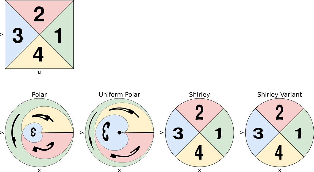
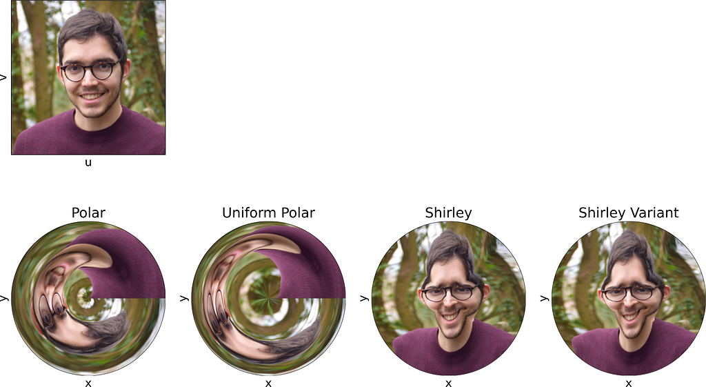
As expected, Shirley’s mapping, when applied to the colored grid, significantly reduces cell stretching and distortion compared to the polar mapping.

Variant of Shirley’s Mapping

The θ mapping in Shirley’s method isn’t very intuitive. Thus, as seen in the figure below, it’s tempting to view it simply as a consequence of the more natural constraint that y depends solely on v, ensuring that horizontal lines remain horizontal.

However, this intuition is incorrect since the horizontal lines are actually slightly curved. The Shirley mapping presented above, i.e. the only uniform mapping respecting the r=u constraint, enforces the following y value, which subtly varies with u.

Although we know it won’t result in a uniform distribution, let’s explore a variant that uses a linear mapping between y and v, just for the sake of experimentation.

The Shirley variant shown here is intended solely for educational purposes, to illustrate how the Shirley mapping alters the horizontal lines by bending them.

We obtain y by scaling v by the length of the half-diagonal, which maps the top-right corner of the square to the edge of the disk. The value of x can then be deduced from y by using the radius constraint r=u.

The figure below shows a side-by-side comparison of the original Shirley mapping and its variant. While both images appear almost identical, it’s worth noting that the variant preserves the horizontality of the lines.

As expected, the empirical density map shows notable deviations from uniformity, oscillating between 0.8 and 1.1 rather than maintaining a constant value of 1.0.

Keep in mind that the density shown below depends on the angle, so the 1D density profile would vary if extracted from a different orientation.

3. Visual Comparison of the sampling methods

Apply the mapping on an image

In the second section of this article, visualizing how a square image is mapped to a disk proved helpful in understanding the distortion caused by the mappings.

To achieve that, we could naively project each colored pixel from the square onto its corresponding location on the disk. However, this approach is flawed, as it doesn’t ensure that every pixel on the disk will be assigned a color. Additionally, some disk pixels may receive multiple colors, resulting in them being overwritten and causing inaccuracies.

The correct approach is to reverse the process: iterate over the disk pixels, apply the inverse mapping to find the corresponding floating-point pixel in the square, and then estimate its color through interpolation. This can be done using cv2.remap from OpenCV.

Thus, the current mapping formulas only allow us to convert disk to square images. To map from square to disk, we need to reverse these formulas.

The inverse formulas are not detailed here for the sake of brevity.

Each of the following subsections will illustrate both the square-to-disk and disk-to-square mappings using a specific pattern image. Enjoy the exploration!

Colored Checkerboard

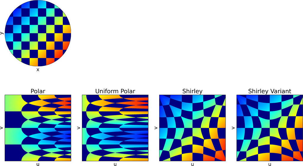
Part of colored Checkerboard

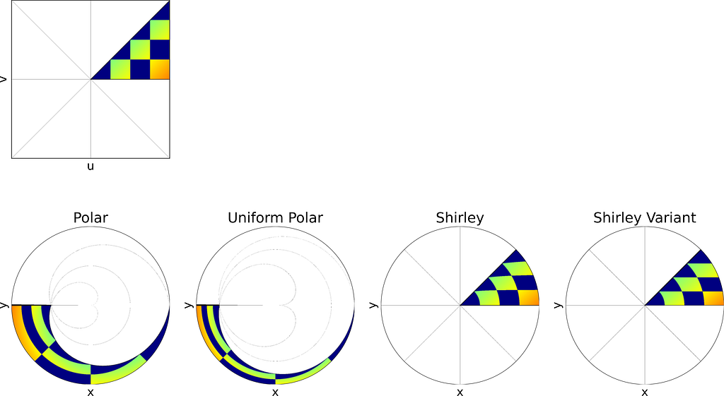
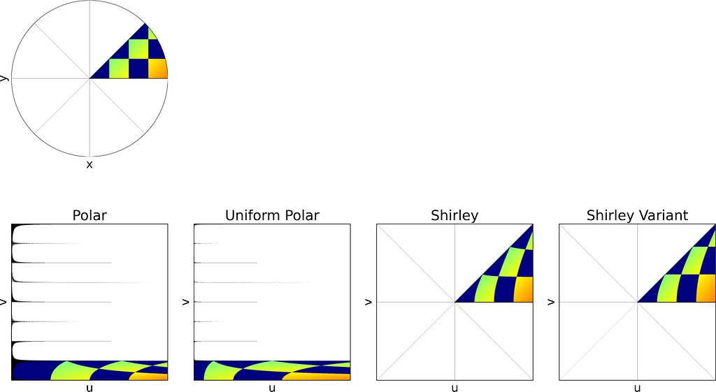
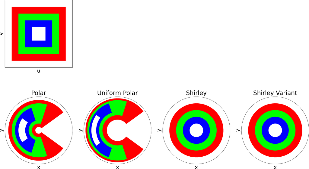
Concentric Squares

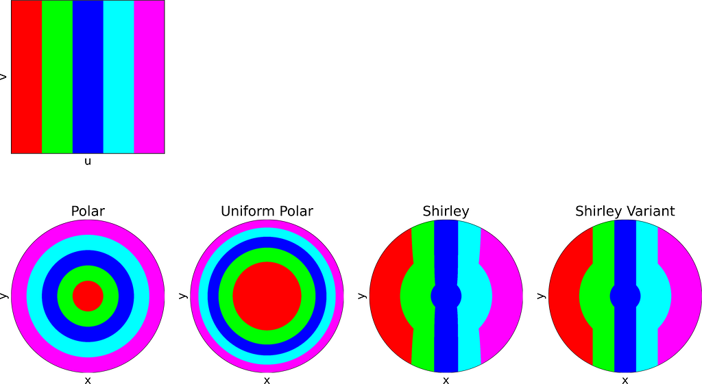
Columns

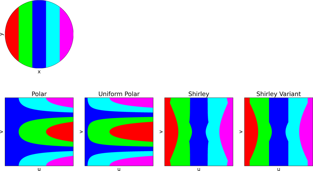
Concentric Circles

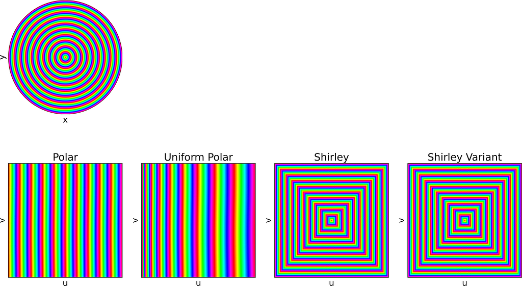
Quadrants

Face

Conclusion

Uniform Sampling

The naive disk sampling approach using uniform polar coordinates is a good example for understanding how transforming variables can affect their distribution.

Using the inversion method you can now turn a uniform sampling on [0,1] into any 1D distribution, by using its inverse Cumulative Distribution Function (CDF).

To sample any 2D distribution, we first sample a variable from its marginal density and then draw the second variable from its conditional density given the first variable.

Distortion and Variance

Depending on your use-case, you might want to guarantee that nearby (u,v) samples will remain close when mapped onto the disk. In such cases, the Shirley transformation is preferable to uniform polar sampling, as it introduces less variance.

Unit Disk Uniform Sampling was originally published in Towards Data Science on Medium, where people are continuing the conversation by highlighting and responding to this story.