Unit Disk and 2D Bounded KDE

How to extend Bounded Kernel Density Estimation to the 2D case? Let’s explore how to fix boundary bias around the unit disk.

0. Introduction

MonteCarlo Integration

Numerical methods become essential when closed-form solutions for integrals are unavailable. While traditional numerical integration techniques like trapezoidal integration are highly effective for low-dimensional and smooth integrals, their efficiency diminishes rapidly, becoming clearly intractable as the dimensionality of the integrand increases.

Unlike traditional techniques, the convergence rate of Monte Carlo methods, which leverage randomness to evaluate integrals, does not depend on the dimensionality of the integrand. It depends solely on the number of random samples drawn.

Sampling

As described in the equation below, the Monte Carlo estimates the integral by a weighted mean of the operand evaluated at samples drawn from a given distribution.

Monte Carlo Integration thus requires to be able to sample from arbitrary distributions across arbitrary dimensions.

With n samples, these methods converge to the correct result at a rate of O(1/sqrt(n)). To halve the error, you need four times as many samples. Therefore, optimizing the sampling process to make the most of each sample is crucial.

Uniform sampling helps ensuring that all regions of the integrand are equally likely to be sampled, avoiding the redundancy of closely spaced samples that provide little additional information.

Other techniques like importance sampling for instance aims at reducing the variance by prioritizing the sampling of more significant regions of the integrand.

Visualize 2D Disk Sampling

The book PBRT (Physically Based Rendering: From Theory To Implementation) does a great job at explaining methods to sample from different geometries like disks, triangles or hemispheres to compute solutions to the integral equations that describe light scattering.

I was excited by the variety of methods I discovered for sampling a disk and intrigued by their underlying principles. To better understand and visually compare these 2D distributions, I decided to plot a density map for each method.

However, a boundary bias occurs when running kernel density estimation (KDE) on a disk because the kernel function extends beyond the boundary of the disk, leading to an underestimation of the density near the edges.

This article aims at providing a way to visualize an unbiased density map of the 2D unit disk.

Article Outline

Building upon my previous article Bounded Kernel Density Estimation, where I explored various methods used to address the boundary bias in the 1D context, we’ll test the following methods:

• Reflection: Reflect points with respect to the circle’s edge
• Transform: Map bounded disk to an unbounded space to perform KDE
• Weighting: Cut and normalize the kernels spreading outside the disk

1. Boundary Bias around the disk

Boundary bias

As As discussed in the introduction, conventional Kernel Density Estimations (KDE) struggle to effectively manage distributions with compact support, such as points within a disk.

Indeed, as illustrated in the figure below with a square domain, kernel span tends to leak beyond the boundary, artificially lowering the density near the edges.

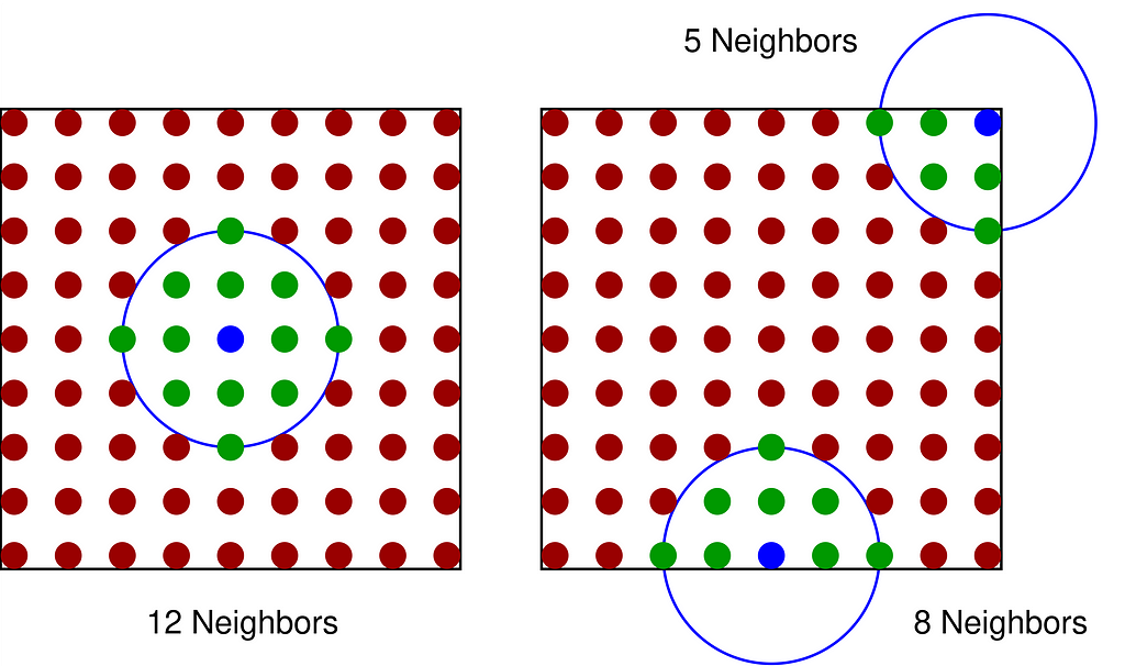
Vanilla Gaussian KDE

The code below samples points on a grid at regular intervals across the unit square, retaining only those within the disk to input into a vanilla Gaussian KDE. Predicted densities are then set to zero outside the disk after the KDE evaluation to keep the boundary constraint.

Finally, the density is normalized by multiplying it by the disk area (π), ensuring an expected density of 1.0 throughout the interior of the disk.

In practice, the input points are not lying on a regular grid, and thus we need to sample a grid at display resolution to evaluate the estimated KDE.

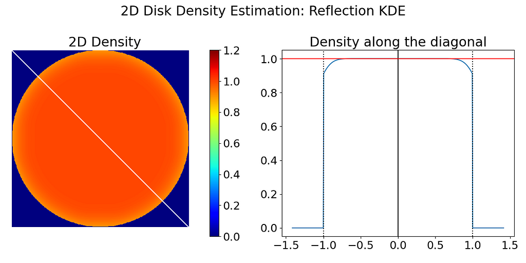
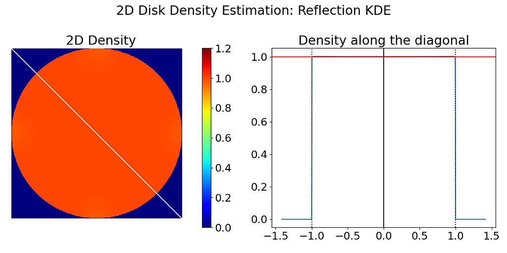
The left figure below has been obtained by running the code above. A noticeable density decrease can be observed around the disk’s edge. To better illustrate the falloff near the edge, I have also extracted the density profile along the diagonal, which ideally should be a perfect step function.

2. Reflection Trick

Reflection

In 1D, the trick consists in augmenting the set of samples by reflecting them across the left and right boundaries. It helps compensating the lack of neighbors on the other side of the boundary. This is equivalent to reflecting the tails of the local kernels to keep them in the bounded domain. The formula below is used to reflect positive 1D values.

Note that it works best when the density derivative is zero at the boundary.

However, in 2D, there isn’t a universal reflection formula; it depends on the boundary shape. Intuitively, the reflection should align with the boundary normals. Therefore, for a disk, it makes sense to reflect points along the radial direction, which means that the reflection only modifies the radius.

Note that handling boundary reflections of the unit square is more challenging than the disk due to the non-differentiability of its boundary line at the corners.

Intuitive Disk Reflection

Intuitively, we can mimic the 1D case by reflecting the point symmetrically across the boundary. A point at radius r is at a distance of 1-r from the edge. By adding this distance beyond the boundary, we get 2-r. The equation and figure below demonstrate how points are reflected across the edge of the unit disk using this symmetry.

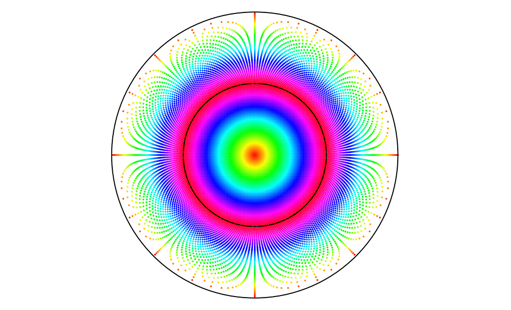
However, when this method is applied to correct the density map, a slight falloff around the edge is still noticeable, although it significantly improves upon the standard KDE.

Optimized Disk Reflection

Let’s see how we can improve this reflection function to better suit the disk boundary. Unlike the 1D case, the f(r)=2-r reflection distorts the space and maps the unit disk of area π to a larger ring of area 3π.

Ideally we’d like that the area of each differential surface inside the disk remains invariant during the reflection mapping. As illustrated in the figure below, we consider differential variations dr and dθ around a point at radius r.

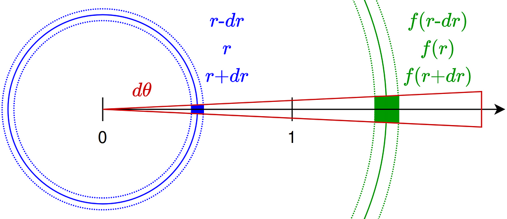
The conservation of area results in a differential equation that the reflection function must satisfy. Note that the minus sign arises because the function f is necessarily decreasing due to its reflective nature.

Given the boundary condition f(1)=1 , there’s a single solution to the differential equation -x=yy’.

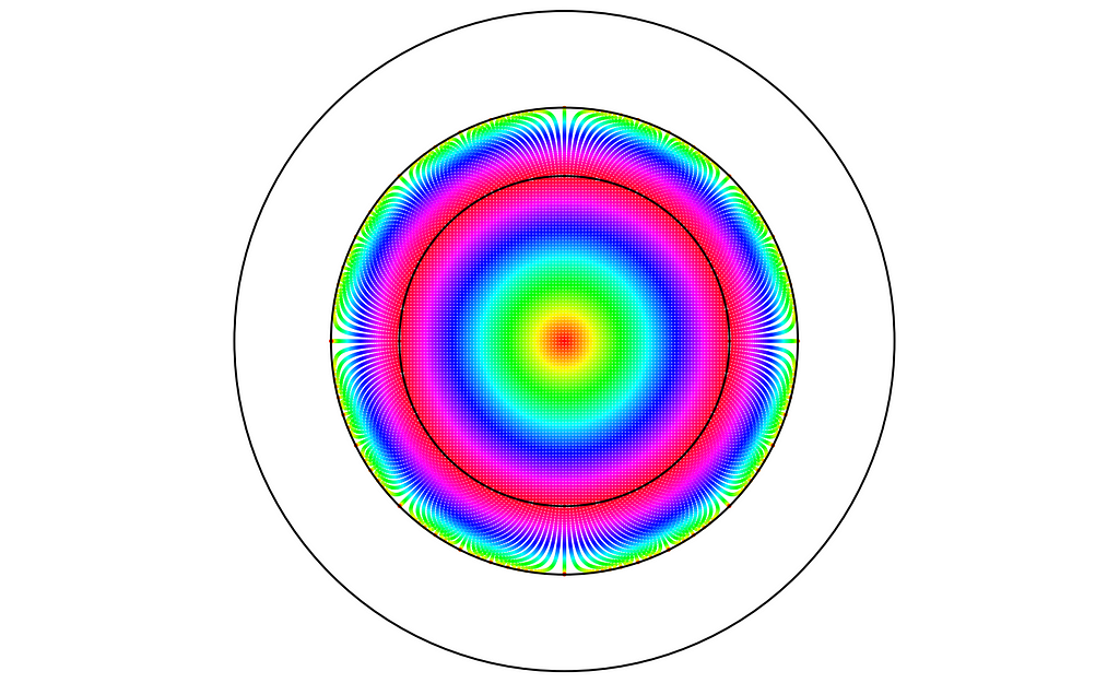
We just have to update our code with the new reflection formula. Reflected points are now contained within the ring between radii 1 and √2. As we can see, reflected points are not too distorted and keep a similar local density.

This time, the resulting density estimate looks nearly perfect!

3. Transformation Trick

KDE in transformed space

The transformation trick maps the bounded data to an unbounded space, where the vanilla KDE can be safely applied. This results in using a different kernel function for each input sample.

However, as seen in previous article Bounded Kernel Density Estimation, , when the density is non-zero at the boundary and does not tend to infinity, it often results in unwanted artifacts.

Transformation

Building upon our approach from the previous section, we will again use central symmetry and choose a transformation f that alters only the radius. Transformed variables will be indicated with a tilde ~.

However, unlike the reflection case, where we preserved the unit disk and used the transformation solely to add new points, here we directly transform and use the points from within the unit disk.

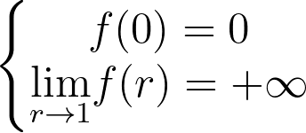
Thus the boundary conditions are different and enforce instead to left the origin untouched and to dilate the disk to infinity.

Density Transformation

When applying a transformation T to a multi-dimensional random variable U, the resulting density is found by dividing by the absolute value of the determinant of the Jacobian matrix of T.

For instance, the polar transformation gives us the following density.

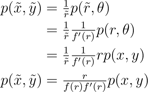
Based on the two previous properties, we can derive the relationship between the density before and after the transformation. This will enable us to recover the true density from the density estimated on the transformed points.

Which transformation to choose? Log, Inverse ?

There are plenty of functions that start from zero and increase to infinity as they approach 1. There is no one-size-fits-all answer.

The figure below showcases potential candidate functions created using logarithmic and inverse transformations to introduce a singularity at r=-1 and r=1.

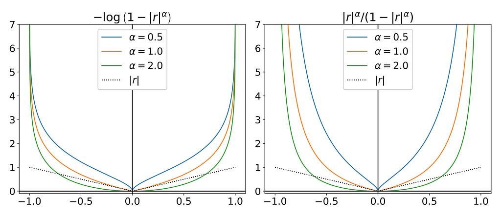
Based on the equation describing the transformed density, we aim to find a transformation that maps the uniform distribution to a form easily estimable by vanilla KDE. If we have a uniform distribution p(x,y), the density in transformed space is thus proportional to the function g below.

Logarithmic and inverse candidates give the following g functions.

They’re both equivalent when r approaches zero and only converge to a meaningful value when α is equal to one.

The figure below illustrates the three cases, with each column corresponding to the log transform with alpha values of 0.5, 1 and 2.

The first row shows the transformed space, comparing the density along the diagonal as estimated by the KDE on the transformed points (blue) against the expected density profile corresponding to the uniform distribution in the original space (red). The second row displays these same curves, but mapped back to the original space.

Keep in mind that the transformation and KDE are still performed in 2D on the disk. The one-dimensional curves shown below are extracted from the 2D results.

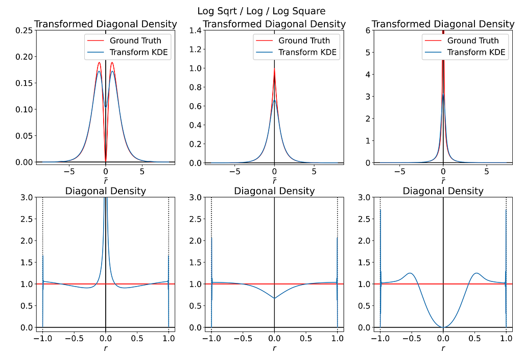
Both α<1 and α>1 introduce singularities near the origin, which completely ruin the interior density estimate. As for α=1, the expected density in transformed space is highly non-differentiable at the origin, resembling a pointed hat shape, which is impossible to fit with gaussian kernels.

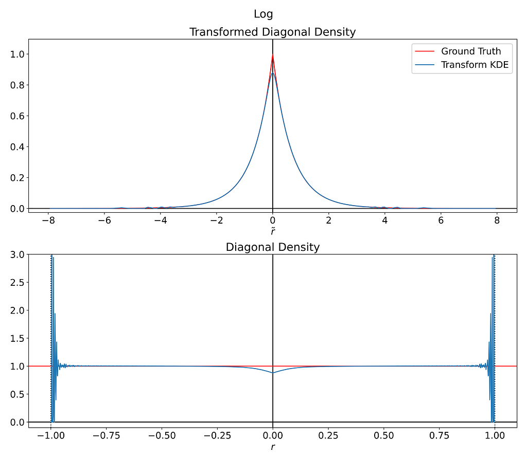
Moreover, the tail density is highly sensible to noise, which can produce high-frequency artifacts near the boundaries. In my opinion, this issue is more problematic than the original bias we are trying to address.

Try with another Kernel?

To achieve more accurate fit for the expected pointed shape when α=1, I estimated the density using a triangular kernel instead of a Gaussian one, as shown in the code below.

Although the fit is slightly better, it remains highly biased at the origin. Additionally, the boundary becomes completely unstable, oscillating at high frequency due to the low bandwidth required to fit the very steep pointed shape at the origin.

Try with the tangent function?

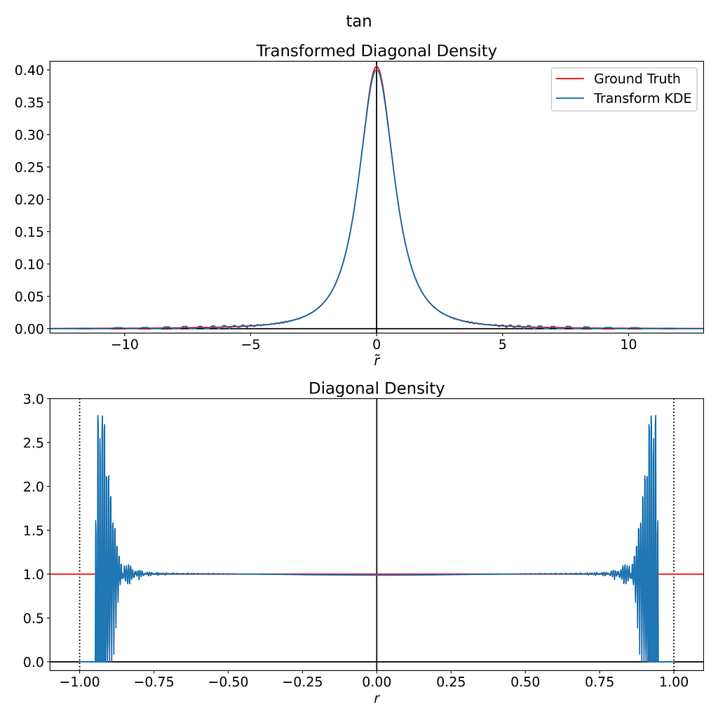
The tangent function also proves to be a suitable candidate to introduce a singularity at r=1.

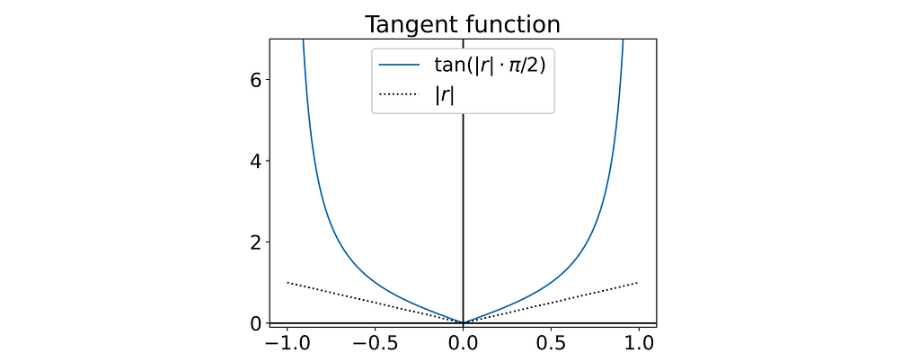
Fortunately, its corresponding g function turns out to be differentiable at the origin, which should make it much easier to fit.

To maintain readability and avoid redundancy, I will not include the mathematical details that led to these results.

However, as illustrated in the figure below, we’re still subject to the same instability around the boundary.

Conclusion

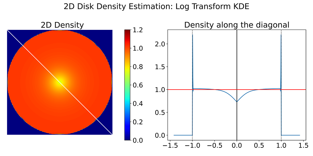
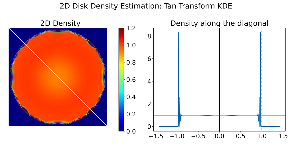
The transformation method appears unsuitable for our uniform distribution within the 2D disk. It introduces excessive variance near the boundaries and significantly disrupts the interior, which was already perfectly unbiased.

Despite the poor performance, I’ve also generated the resulting 2D density map obtained with the Transform KDE using the log and tangent transformations.

4. Cut-and-Normalize Trick

Weighting

Since the density is artificially lower around he boundary because of the lack of neighbors, we could compute how much of our local kernel has been lost outside the bounded domain and leverage it to correct the bias.

In 1D, this involves computing the integral of a Gaussian over an interval. It’s straightforward, as it can be done by estimating the Cumulative Density Function at both ends of the interval and subtracting the values.

However, in 2D, this requires computing the integral of a 2D Gaussian over a disk. Since there is no analytical solution for this, it must be numerically approximated, making it more computationally expensive.

Numerical Approximation

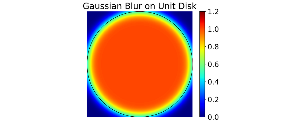
It would be too expensive to perform numerical integration for each single predicted density. Since we are essentially computing the convolution between a binary disk and a Gaussian kernel, I propose discretizing the unit square to perform numerical convolution.

In the code below, we assume an isotropic Gaussian and retrieve the kernel standard deviation. Subsequently, we perform the convolution on the binary disk mask using OpenCV, resulting in the array shown in the figure below. Notice how closely it approximates the biased vanilla KDE.

Result

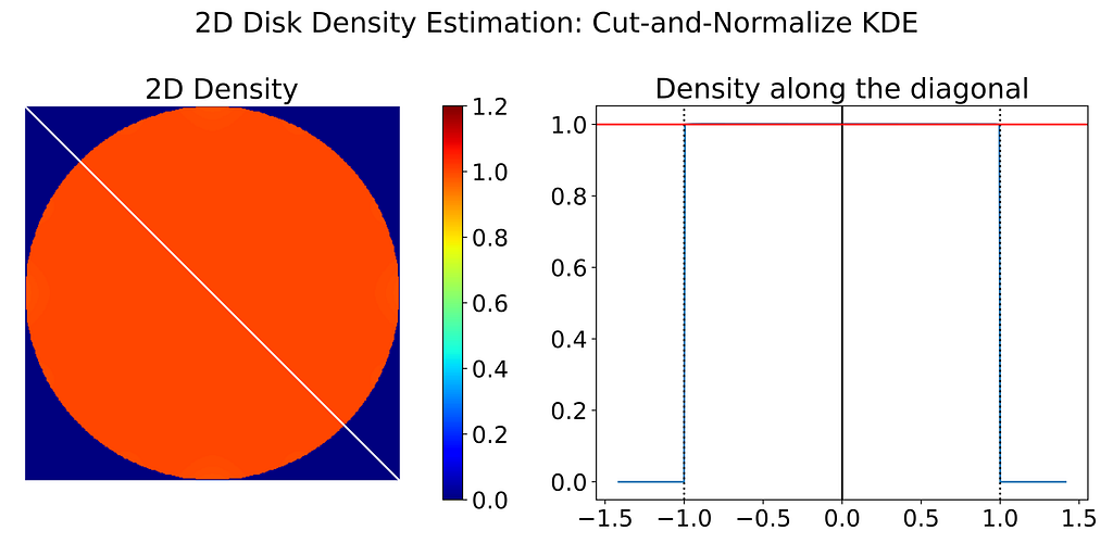
Once the correction weight map has been computed, we can apply it to the biased predicted density. The corrected density map is then almost perfect.

Conclusion

Performance

The Reflection and Cut-and-Normalize methods are very easy to use and effectively mitigate the boundary bias. In contrast, the Transform method shows poor performance on the uniform 2D disk, despite testing various singular functions and kernel types.

Speed

The Reflection method transforms the input of the KDE, whereas the Cut-and-Normalize method transforms its output.

Since the Gaussian KDE has a time complexity that is quadratic in the number of samples, i.e. O(n²), Reflection is approximately four times slower than Cut-and-Normalize because it requires twice as many samples.

Thus, the Cut-and-Normalize method seems to be the easiest and fastest way to compensate the boundary bias on the 2D uniform Disk distribution.

Visualize 2D Disk Sampling

We can now simulate different disk sampling strategies and compare them based on their density map, without having to worry about the boundary bias.

I hope you enjoyed reading this article and that it gave you more insights on how to perform bounded Kernel Density Estimation in the 2D case.

Unit Disk and 2D Bounded KDE was originally published in Towards Data Science on Medium, where people are continuing the conversation by highlighting and responding to this story.