Understanding Transformers

A straightforward breakdown of “Attention is All You Need”¹

The transformer came out in 2017. There have been many, many articles explaining how it works, but I often find them either going too deep into the math or too shallow on the details. I end up spending as much time googling (or chatGPT-ing) as I do reading, which isn’t the best approach to understanding a topic. That brought me to writing this article, where I attempt to explain the most revolutionary aspects of the transformer while keeping it succinct and simple for anyone to read.

This article assumes a general understanding of machine learning principles.

The ideas behind the Transformer led us to the era of Generative AI

Transformers represented a new architecture of sequence transduction models. A sequence model is a type of model that transforms an input sequence to an output sequence. This input sequence can be of various data types, such as characters, words, tokens, bytes, numbers, phonemes (speech recognition), and may also be multimodal¹.

Before transformers, sequence models were largely based on recurrent neural networks (RNNs), long short-term memory (LSTM), gated recurrent units (GRUs) and convolutional neural networks (CNNs). They often contained some form of an attention mechanism to account for the context provided by items in various positions of a sequence.

The downsides of previous models

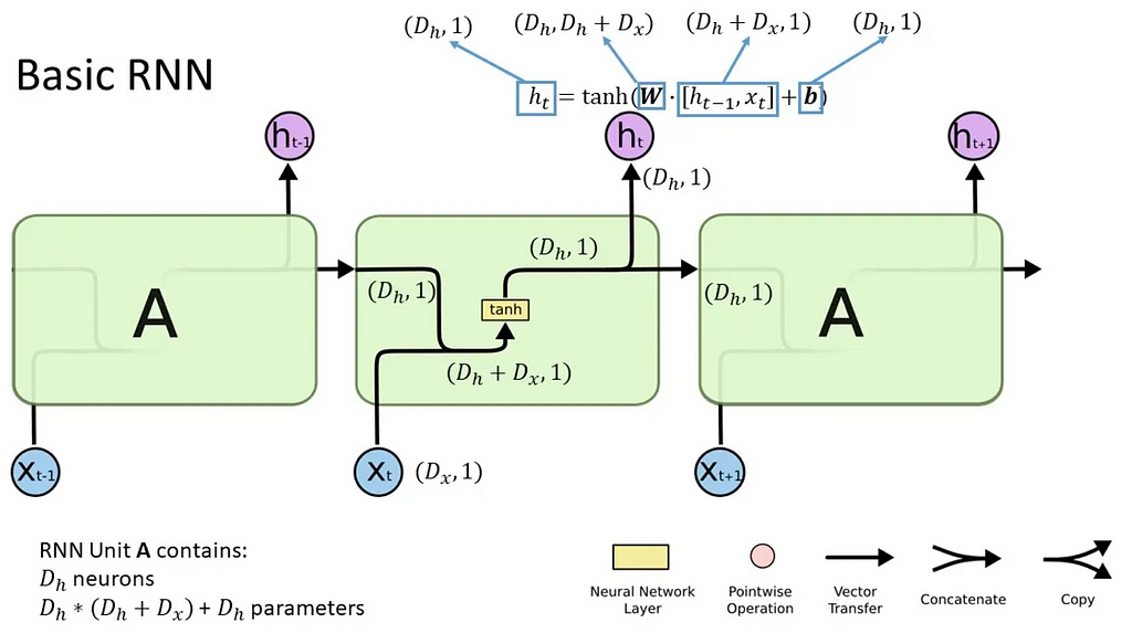
• RNNs: The model tackles the data sequentially, so anything learned from the previous computation is accounted for in the next computation². However, its sequential nature causes a few problems: the model struggles to account for long-term dependencies for longer sequences (known as vanishing or exploding gradients), and prevents parallel processing of the input sequence as you cannot train on different chunks of the input at the same time (batching) because you will lose context of the previous chunks. This makes it more computationally expensive to train.

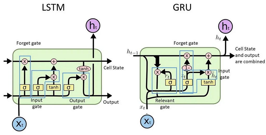
• LSTM and GRUs: Made use of gating mechanisms to preserve long-term dependencies³. The model has a cell state which contains the relevant information from the whole sequence. The cell state changes through gates such as the forget, input, output gates (LSTM), and update, reset gates (GRU). These gates decide, at each sequential iteration, how much information from the previous state should be kept, how much information from the new update should be added, and then which part of the new cell state should be kept overall. While this improves the vanishing gradient issue, the models still work sequentially and hence train slowly due to limited parallelisation, especially when sequences get longer.
• CNNs: Process data in a more parallel fashion, but still technically operates sequentially. They are effective in capturing local patterns but struggle with long-term dependencies due to the way in which convolution works. The number of operations to capture relationships between two input positions increases with distance between the positions.

Hence, introducing the Transformer, which relies entirely on the attention mechanism and does away with the recurrence and convolutions. Attention is what the model uses to focus on different parts of the input sequence at each step of generating an output. The Transformer was the first model to use attention without sequential processing, allowing for parallelisation and hence faster training without losing long-term dependencies. It also performs a constant number of operations between input positions, regardless of how far apart they are.

Walking through the Transformer model architecture

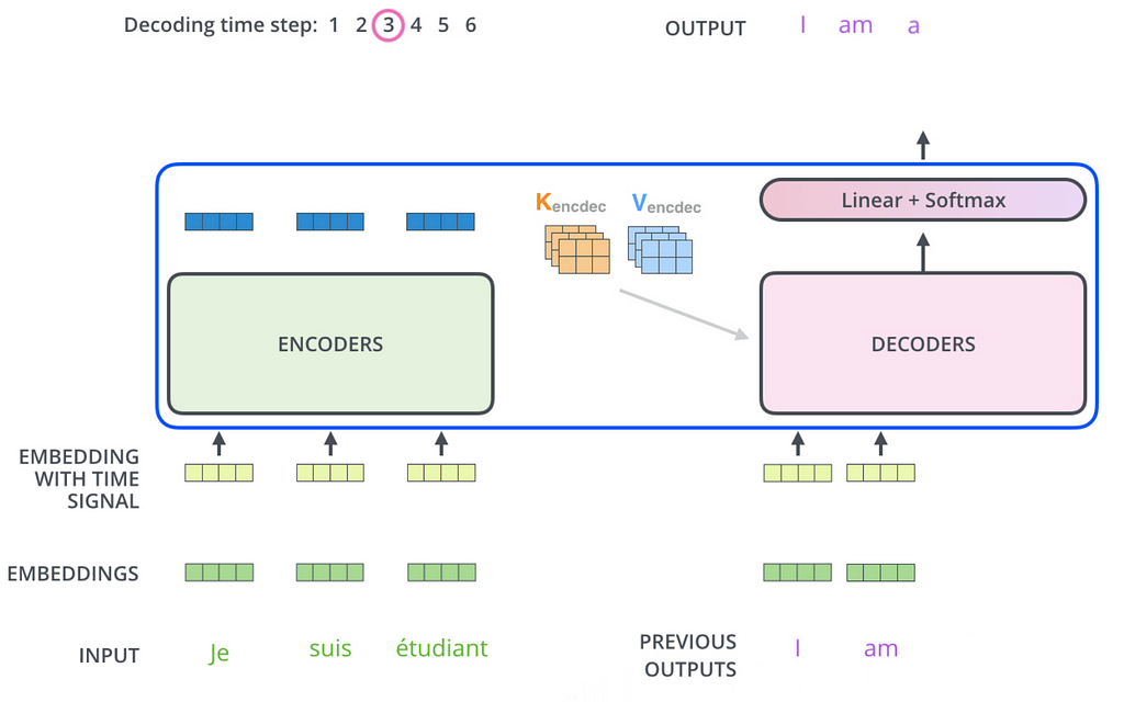
The important features of the transformer are: tokenisation, the embedding layer, the attention mechanism, the encoder and the decoder. Let’s imagine an input sequence in french: “Je suis etudiant” and a target output sequence in English “I am a student” (I am blatantly copying from this link, which explains the process very descriptively)

Tokenisation

The input sequence of words is converted into tokens of 3–4 characters long

Embeddings

The input and output sequence are mapped to a sequence of continuous representations, z, which represents the input and output embeddings. Each token will be represented by an embedding to capture some kind of meaning, which helps in computing its relationship to other tokens; this embedding will be represented as a vector. To create these embeddings, we use the vocabulary of the training dataset, which contains every unique output token that is being used to train the model. We then determine an appropriate embedding dimension, which corresponds to the size of the vector representation for each token; higher embedding dimensions will better capture more complex / diverse / intricate meanings and relationships. The dimensions of the embedding matrix, for vocabulary size V and embedding dimension D, hence becomes V x D, making it a high-dimensional vector.

At initialisation, these embeddings can be initialised randomly and more accurate embeddings are learned during the training process. The embedding matrix is then updated during training.

Positional encodings are added to these embeddings because the transformer does not have a built-in sense of the order of tokens.

Attention mechanism

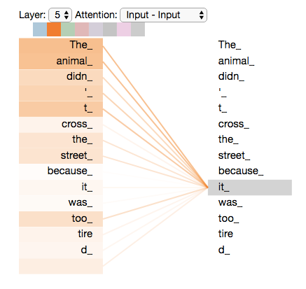
Self-attention is the mechanism where each token in a sequence computes attention scores with every other token in a sequence to understand relationships between all tokens regardless of distance from each other. I’m going to avoid too much math in this article, but you can read up here about the different matrices formed to compute attention scores and hence capture relationships between each token and every other token.

These attention scores result in a new set of representations⁴ for each token which is then used in the next layer of processing. During training, the weight matrices are updated through back-propagation, so the model can better account for relationships between tokens.

Multi-head attention is just an extension of self-attention. Different attention scores are computed, the results are concatenated and transformed and the resulting representation enhances the model’s ability to capture various complex relationships between tokens.

Encoder

Input embeddings (built from the input sequence) with positional encodings are fed into the encoder. The input embeddings are 6 layers, with each layer containing 2 sub-layers: multi-head attention and feed forward networks. There is also a residual connection which leads to the output of each layer being LayerNorm(x+Sublayer(x)) as shown. The output of the encoder is a sequence of vectors which are contextualised representations of the inputs after accounting for attention scored. These are then fed to the decoder.

Decoder

Output embeddings (generated from the target output sequence) with positional encodings are fed into the decoder. The decoder also contains 6 layers, and there are two differences from the encoder.

First, the output embeddings go through masked multi-head attention, which means that the embeddings from subsequent positions in the sequence are ignored when computing the attention scores. This is because when we generate the current token (in position i), we should ignore all output tokens at positions after i. Moreover, the output embeddings are offset to the right by one position, so that the predicted token at position i only depends on outputs at positions less than it.

For example, let’s say the input was “je suis étudiant à l’école” and target output is “i am a student in school”. When predicting the token for student, the encoder takes embeddings for “je suis etudiant” while the decoder conceals the tokens after “a” so that the prediction of student only considers the previous tokens in the sentence, namely “I am a”. This trains the model to predict tokens sequentially. Of course, the tokens “in school” provide added context for the model’s prediction, but we are training the model to capture this context from the input token,“etudiant” and subsequent input tokens, “à l’école”.

How is the decoder getting this context? Well that brings us to the second difference: The second multi-head attention layer in the decoder takes in the contextualised representations of the inputs before being passed into the feed-forward network, to ensure that the output representations capture the full context of the input tokens and prior outputs. This gives us a sequence of vectors corresponding to each target token, which are contextualised target representations.

The prediction using the Linear and Softmax layers

Now, we want to use those contextualised target representations to figure out what the next token is. Using the contextualised target representations from the decoder, the linear layer projects the sequence of vectors into a much larger logits vector which is the same length as our model’s vocabulary, let’s say of length L. The linear layer contains a weight matrix which, when multiplied with the decoder outputs and added with a bias vector, produces a logits vector of size 1 x L. Each cell is the score of a unique token, and the softmax layer than normalises this vector so that the entire vector sums to one; each cell now represents the probabilities of each token. The highest probability token is chosen, and voila! we have our predicted token.

Training the model

Next, we compare the predicted token probabilities to the actual token probabilites (which will just be logits vector of 0 for every token except for the target token, which has probability 1.0). We calculate an appropriate loss function for each token prediction and average this loss over the entire target sequence. We then back-propagate this loss over all the model’s parameters to calculate appropriate gradients, and use an appropriate optimisation algorithm to update the model parameters. Hence, for the classic transformer architecture, this leads to updates of

1. The embedding matrix
2. The different matrices used to compute attention scores
3. The matrices associated with the feed-forward neural networks
4. The linear matrix used to make the logits vector

Matrices in 2–4 are weight matrices, and there are additional bias terms associated with each output which are also updated during training.

Note: The linear matrix and embedding matrix are often transposes of each other. This is the case for the Attention is All You Need paper; the technique is called “weight-tying”. The number of parameters to train are thus reduced.

This represents one epoch of training. Training comprises multiple epochs, with the number depending on the size of the datasets, size of the models, and the model’s task.

Going back to what makes Transformers so good

As we mentioned earlier, the problems with the RNNs, CNNs, LSTMs and more include the lack of parallel processing, their sequential architecture, and inadequate capturing of long-term dependencies. The transformer architecture above solves these problems as…

1. The Attention mechanism allows the entire sequence to be processed in parallel rather than sequentially. With self-attention, each token in the input sequence attends to every other token in the input sequence (of that mini batch, explained next). This captures all relationships at the same time, rather than in a sequential manner.
2. Mini-batching of input within each epoch allows parallel processing, faster training, and easier scalability of the model. In a large text full of examples, mini-batches represent a smaller collection of these examples. The examples in the dataset are shuffled before being put into mini-batches, and reshuffled at the beginning of each epoch. Each mini-batch is passed into the model at the same time.
3. By using positional encodings and batch processing, the order of tokens in a sequence is accounted for. Distances between tokens are also accounted for equally regardless of how far they are, and the mini-batch processing further ensures this.

As shown in the paper, the results were fantastic.

Welcome to the world of transformers.

A quick bit on GPT Architecture

The transformer architecture was introduced by the researcher Ashish Vaswani in 2017 while he was working at Google Brain. The Generative Pre-trained Transformer (GPT) was introduced by OpenAI in 2018. The primary difference is that GPT’s do not contain an encoder stack in their architecture. The encoder-decoder makeup is useful when were directly converting one sequence into another sequence. The GPT was designed to focus on generative capabilities, and it did away with the decoder while keeping the rest of the components similar.

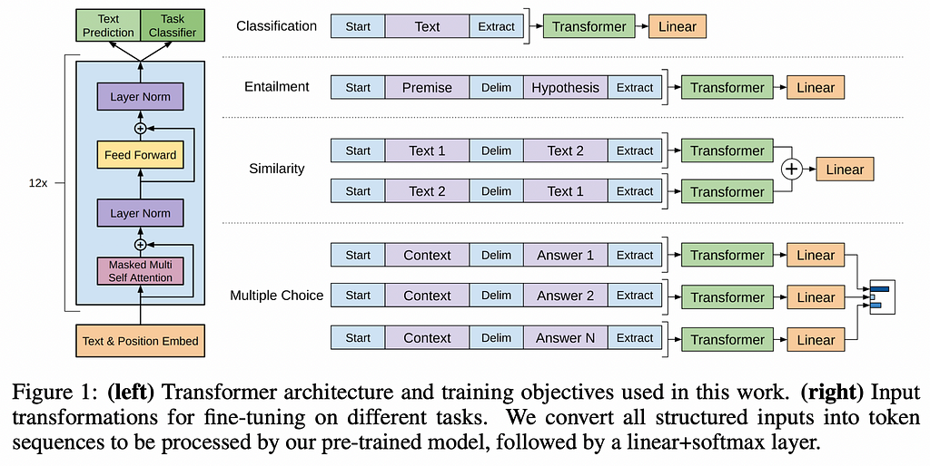
The GPT model is pre-trained on a large corpus of text, unsupervised, to learn relationships between all words and tokens⁵. After fine-tuning for various use cases (such as a general purpose chatbot), they have proven to be extremely effective in generative tasks.

Example

When you ask it a question, the steps for prediction are largely the same as a regular transformer. If you ask it the question “How does GPT predict responses”, these words are tokenised, embeddings generated, attention scores computed, probabilities of the next word are calculated, and a token is chosen to be the next predicted token. For example, the model might generate the response step by step, starting with “GPT predicts responses by…” and continuing based on probabilities until it forms a complete, coherent response. (guess what, that last sentence was from chatGPT).

I hope all this was easy enough to understand. If it wasn’t, then maybe it’s somebody else’s turn to have a go at explaining transformers.

Feel free to share your thoughts and connect with me if this article was interesting to you!

• LinkedIn: https://www.linkedin.com/in/aveekg00/
• Website: aveek.info

References:

1. https://arxiv.org/pdf/1706.03762
2. https://deeplearningmath.org/sequence-models
3. http://colah.github.io/posts/2015-08-Understanding-LSTMs/
4. http://jalammar.github.io/illustrated-transformer/
5. https://openai.com/index/language-unsupervised/

Other great articles to refer to:

• https://lilianweng.github.io/posts/2018-06-24-attention/
• https://bastings.github.io/annotated_encoder_decoder/
• https://nlp.seas.harvard.edu/annotated-transformer/#prelims

Understanding Transformers was originally published in Towards Data Science on Medium, where people are continuing the conversation by highlighting and responding to this story.