Towards Monosemanticity: A step towards understanding large language models

Towards Monosemanticity: A Step Towards Understanding Large Language Models

Understanding the mechanistic interpretability research problem and reverse-engineering these large language models

Context

One of AI researchers’ main burning questions is understanding how these large language models work. Mathematically, we have a good answer on how different neural network weights interact and produce a final answer. But, understanding them intuitively is one of the core questions AI researchers aim to answer. It is important because unless we understand how these LLMs work, it is very difficult to solve problems like LLM alignment and AI safety or to model the LLM to solve specific problems. This problem of understanding how large language models work is defined as a mechanistic interpretability research problem and the core idea is how we can reverse-engineer these large language models.

Anthropic is one of the companies that has made great strides in understanding these large models. The main question is how these models work apart from a mathematical point of view. In Oct ’23, they published this paper: Towards Monosemanticity: Decomposing Language models with dictionary learning (link). This paper aims to solve this problem and build a basic understanding of how these models work.

The below post aims to capture high-level basic concepts and build a solid foundation to understand the “Towards Monosemanticity: Decomposing Language Models with dictionary learning” paper.

The paper starts with a loaded term, “Towards Monosemanticity”. Let’s dive straight into it to understand what this means.

What is Monosemanticity vs Polysemanticity?

The basic unit of a large language model is a neural network which is made of neurons. So, neurons are the basic unit of the entire LLM’s. However, on inspection, we find that neurons fire for unrelated concepts in neural networks. For example: For vision models, a single neuron responds to “faces of cats” as well as “fronts of cars”. This concept is called “polysemantic”. This means neurons can respond to mixtures of unrelated inputs. This makes this problem very hard since the neuron itself cannot be used to analyze the behavior of the model. It would be nice if one neuron responds to the faces of cats while another neuron responds to the front of cars. If a neuron only fires for one feature, this property would have been called “monosemanticity”.

Hence the first section of the paper, “Towards Monosemanticity,” means if we can move from polysemanticity towards monosemanticity, this can help us understand neural networks with better depth.

How to go further beyond neurons

Now, the key question is if neurons fire for unrelated concepts, it means there needs to be a more fundamental representation of data that the network learns. Let’s take an example: “Cats” and “Cars”. Cats can be represented as a combination of “animal, fur, eyes, legs, moving” while Cars can be a combination of “wheels, seats, rectangle, headlight”. This is 1st level representation. These can be further broken down into abstract concepts. Let’s take “eyes” and “headlight”. Eyes can be represented as “round, black, white” while headlight can be represented as “round, white, light”. As you can see, we can further build this abstract representation and notice that two very unrelated things (Cat and Car) start to share some representations. This is only 2 layers deep and can be imagined if we represent 8x, 16x, or 256x layers deep. A lot of things will be represented with very basic abstract concepts (difficult to interpret for humans) but concepts will be shared among different entities.

The author uses terminology called “features” to represent this concept. According to the paper, each neuron can store many unrelated features and hence fires for completely unrelated inputs.

If a neuron is storing many features, how to get feature-level representation?

The answer is always to scale more. If we think about this as if a neuron is storing, let’s say, 5 different features, can we break the neuron into 5 individual neurons and have each sub-neuron represent features? This is the core idea behind the paper.

The below image is a representation of the core idea of the paper. The “Observed model” is the actual model that stores multiple features of information. It is called the low-dimensional projection of some hypothetical larger network. The larger network is a hypothetical disentangled model that represents each neuron mapping to one feature and showing “monosemanticity” behavior.

With this, we can say whatever model we trained on, there will always be a bigger model that can contain 1:1 mapping between data and feature and hence we need to learn this bigger model for moving towards monosemanticity.

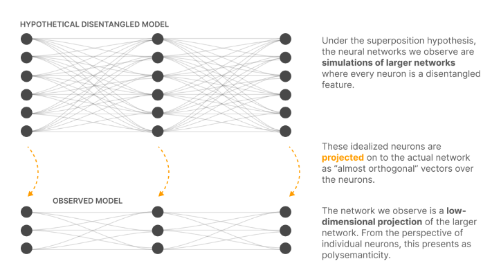
Now, before moving to technical implementation, let’s review all the information so far. The neuron is the basic unit in neural networks but contains multiple features of data. When data (tokens) are broken down into smaller abstract concepts, these are called features. If a neuron is storing multiple features, we need a way to represent each feature with its neuron so that only one neuron fires for each feature. This approach will help us move towards “monosemanticity”. Mathematically, it means we need to scale more as we need more neurons to represent the data into features.

With the basic and core idea under our grasp, let’s move to the technical implementation of how such things can be built.

Technical setup

Since we have established we need more scaling, the idea is to scale up the output after multi-layer perceptron (MLP). Before moving on to how to scale, let’s quickly review how the LLM model works with transformer and MLP blocks.

The below image is a representation of how the LLM model works with a transformer and MLP block. The idea is that each token is represented in terms of embeddings (vector) and is passed to the attention block which computes attention across different tokens. The output of the attention block is the same dimension as the input of each token. Now the output of each token from the attention block is parsed through a multi-layer perceptron (MLP) which scales up and then scales down the token to the same size as the input token. This step is repeated multiple times before the final output. In the case of chat-GPT-3, 96 layers do this operation. This is the same as how the transformer architecture works. Refer to the “Attention is all you need” paper for more details. Link

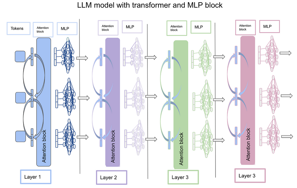
Now with the basic architecture laid out, let’s delve deeper into what sparse autoencoders are. The authors used “sparse autoencoders” to do up and down scaling and hence these have become a fundamental block to understand.

Sparse auto-encoders

Sparse auto-encoders are the neural network itself but contain 3 stages of the neural network (encoder, sparse activation in the middle, and decoder). The idea is that the auto-encoder takes, let’s say, 512-dimensional input, scales to a 4096 middle layer, and then reduces to 512-dimensional output. Now once an input of 512 dimensions comes, it goes through an encoder whose job is to isolate features from data. After this, it is mapped into high dimensional space (sparse autoencoder activations) where only a few non-zero values are allowed and hence considered sparse. The idea here is to force the model to learn a few features in high-dimensional space. Finally, the matrix is forced to map back into the decoder (512 size) to reconstruct the same size and values as the encoder input.

The below image represents the sparse auto-encoder (SAE) architecture.

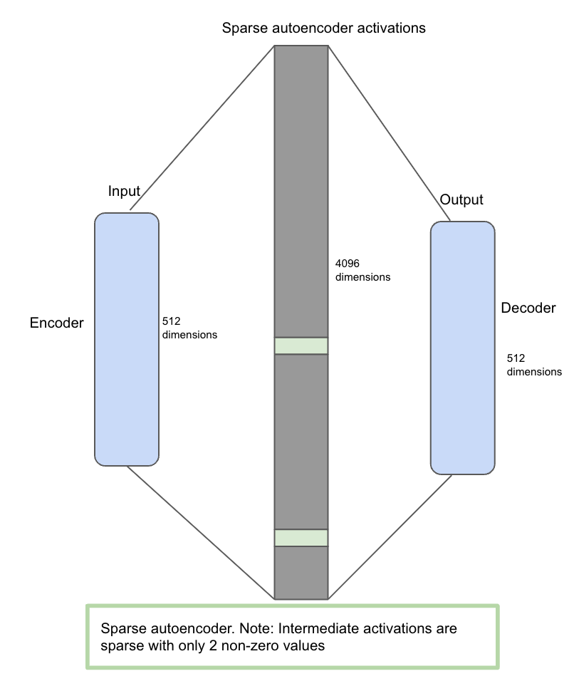
With basic transformer architecture and SAE explained, let’s try to understand how SAE’s are integrated with transformer blocks for interpretability.

How is sparse auto-encoder (SAE) integrated with an LLM?

An LLM is based on a transformer block which is an attention mechanism followed by an MLP (multi-layer perceptron) block. The idea is to take output from MLP and feed it into the sparse auto-encoder block. Let’s take an example: “Golden Gate was built in 1937”. Golden is the 1st token which gets parsed through the attention block and then the MLP block. The output after the MLP block will be the same dimension as input but it will contain context from other words in the sentence due to attention mechanisms. Now, the same output vector from the MLP block becomes the input of the sparse auto-encoder itself. Each token has its own MLP output dimensions which can be fed into SAE as well. The below diagram conveys this information and how it is integrated with the transformer block.

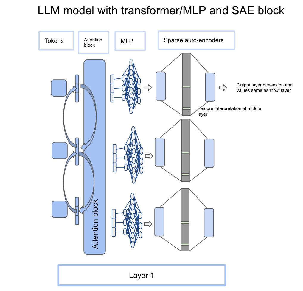
Side note: The below image is very famous in the paper and conveys the same information as the above section. It takes input from the activation vector from the MLP layer and feeding into SAE for feature scaling. Hopefully, the image below will make a lot more sense with the above explanation.

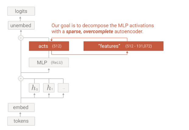
Now, that we understand the architecture and integration of SAE with LLM’s, the basic question is how are these SAE trained? Since these are also neural networks, these models need to be trained as well.

How are autoencoders trained?

The dataset for autoencoders comes from the main LLM itself. When training an LLM model with a token, the output after every MLP layer called activation vectors is stored for each token. So we have an input of tokens (512 size) and an output from MLP activation layer (512 size). We can collect different activations for the same tokens in different contexts. In the paper, the author collected different activations for 256 contexts for the same token. This gives a good representation of a token in different context settings.

Once the input is selected, SAE is trained for input and output (input is same as output from MLP activation layer (512 size), output is same as input). Since input is equal to output, the job of SAE is to enhance the information of 512 size to 4096 size with sparse activation (1–2 non-zero values) and then convert back to 512 size. Since it is upscaling but with a penalty to reconstruct the information with 1–2 non-zero values, this is where the learning happens and the model is forced to learn 1–2 features for a specific data/token.

Intuitively, this is a very simple problem for a model to learn. The input is the same as output and the middle layer is larger than the input and output layer. The model can learn the same mapping but we introduce a penalty for only a few values in the middle layer that are non-zero. Now it becomes a difficult problem since input is the same as output but the middle layer has only 1–2 non-zero values. So the model has to explicitly learn in the middle layer of what the data represents. This is where data gets broken down into features and features are learned in the middle layer.

With all this understanding, we are ready to tackle feature interpretability now.

Feature interpretability

Since training is done, let’s move to the inference phase now. This is where the interpretation begins now. The output from the MLP layer of the LLM’s model is fed into the SAE. In the SAE, only a few (1–2) blocks become activated. This is the middle layer of the SAE. Here, human inspection is required to see what neuron in the middle layer gets activated.

Example: Let’s say there are 2 types of context given to LLM and our job is to figure out when “Golden” is triggered. Context 1: “Golden Gate was built in 1937”, Context 2: “Golden Gate is in San Francisco”. When both the contexts are fed into LLM and the output of context 1 and context 2 for the “Golden” token is taken and fed into SAE, there should be only 1–2 features fired in the middle layer of SAE. Let’s say this feature number is 1345(a random number assigned out of 4096). This will denote that the 1345 feature gets triggered when Golden Gate is mentioned in the token input list. This means feature 1345 represents the “Golden Gate” context.

Hence, this is one way to interpret features from SAE.

Limitations of the current approach

Measurement: The main bottleneck comes around the interpretation of the features. In the above example, human judgment is required to see if 1345 belongs to Golden Gate and is tested with multiple contexts. No mathematical loss function formulation helps answer this question quantitatively. This is one of the main bottlenecks that mechanistic interpretability faces in determining how to measure whether the progress of machines is interpretable or not.

Scaling: Another aspect is scaling, since training SAE on each layer with 4x more parameters is extremely memory and computation-intensive. As main models increase their parameters, it becomes even more difficult to scale SAE and hence there are concerns around the scaling aspect of using SAE as well.

But overall, this has been a fascinating journey. We started from a model and understood their nuances around interpretability and why neurons, despite being a basic unit, are still not the fundamental unit to understand. We went deeper to understand how data is made up of features and if there is a way to learn features. We learned how sparse auto-encoders help learn the sparse representation of the features and can be the building block of feature representation. Finally, we learned how to train sparse auto-encoders and after training, how SAE’s can be used to interpret the features in the inference phase.

Conclusion

The field of mechanistic interpretability has a long way to go. However current research from Anthropic in terms of introducing sparse auto-encoders is a big step towards interpretability. The field still suffers from limitations around measurement and scaling challenges but so far has been one of the best and most advanced research in the field of mechanistic interpretability.

References

• https://transformer-circuits.pub/2023/monosemantic-features
• https://www.lesswrong.com/posts/CJPqwXoFtgkKPRay8/an-intuitive-explanation-of-sparse-autoencoders-for
• https://www.dwarkeshpatel.com/p/dario-amodei

Towards Monosemanticity: A step towards understanding large language models was originally published in Towards Data Science on Medium, where people are continuing the conversation by highlighting and responding to this story.