The Math Behind Risk — Part 2
Does the attack really have an advantage in the game of world conquest?
In Part 1, we discussed the relative chances for attack and defense in Risk, the game of world conquest. At the end of Part 1, we concluded that the attack has a 47.15% chance of winning the battle for the first soldier and we wondered how the famous conquerors were able to achieve their feats under these conditions. We saved the discussion of the second soldier for Part 2.

To refresh our memories, in Risk, the attack rolls up to 3 dice, while the defense rolls up to 2 dice. The highest rolls of each are compared and the loser loses a soldier, with the defense winning in the case of a tie. Next, the second highest rolls of each are compared, and once again, the loser loses a soldier, with the defense winning in the case of a tie once again.
Well, here we are. Let’s dive into it.
(Here you can find code in which I confirm the below probabilities.)
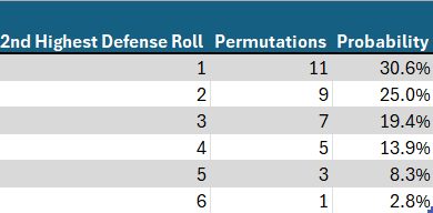
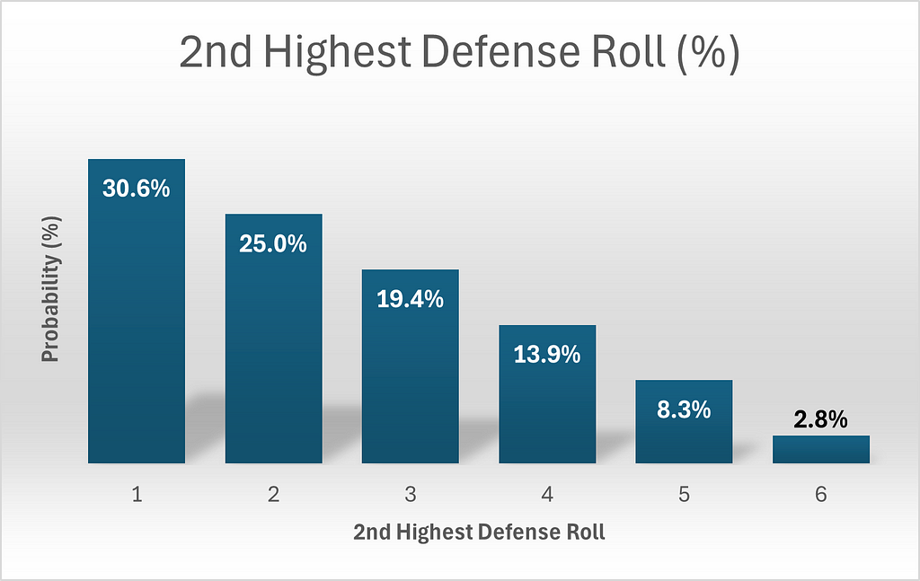
Of course, regarding the defender’s probabilities, we are merely calculating the lowest roll, since he has only two dice. Therefore, the probabilities are a mirror image of the probabilities we saw regarding the highest roll. This time, there are 11 possibilities yielding a 2nd highest roll of 1, 9 for 2, 7 for 3 etc. The probability can be calculated by dividing by 36, the total number of permutations possible for the two dice of the defense.
Calculating the second highest roll among the three dice of the attacker differs significantly from the calculations of Part 1. I’ll be honest. I struggled with this a little. In the calculations that follow, two things must be borne in mind.
- We must consider both how many outcomes are possible and how many ways in which each outcome can occur. For example, an outcome of (6, 2, 3) is of course a single outcome, but it can occur in 6 ways, corresponding to which die each value occurs on. It can be any of {(2, 3, 6), (2, 6, 3), (3, 2, 6), (3, 6, 2), (6, 2, 3), (6, 3, 2)}. This outcome therefore corresponds to 1*6 = 6 permutations. For another example, an outcome with exactly two ones is actually a collection of 5 outcomes, since the remaining die can take any value between 2 and 6. And it can occur in any of 3 ways, {(1, 1, x), (1, x, 1), (x, 1, 1)}, corresponding to the 3 possible locations for the remaining die, so this outcome actually corresponds to 5*3 = 15 permutations.
- We must be careful with doubles and triples. These must be considered separately since, while there are 6 ways to obtain an outcome of (1, 2, 3), there are only 3 ways to obtain a (1, 2, 2) and only 1 way to obtain a (2, 2, 2).
With the above considerations in mind, we are ready to proceed.
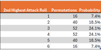
Consider the probability of getting a 2nd highest roll of 1. This is relatively straight-forward. Clearly the lowest roll is a 1 as well. For now, we will disregard the case where all 3 dice are 1. The highest die can then take any value between 2and 6, and it can appear upon any of the 3 dice, since we have not specified which of the 3 dice contains the highest roll. This yields a total of 3*5=15 permutations. Adding the case of a triple 1 yields a total of 16 permutations. By a symmetrical argument, we can calculate that the same number of permutations yield a 2nd highest roll of 6.
Next, what about getting a 2 as the second highest roll? For now, we will disregard the possibility of multiple twos and assume that the highest roll was higher than 2 and that the lowest roll was lower than 2. The highest roll can take 4 values (3–6) and the lowest toll must be 1, for a total of 4 outcomes, and these can occur at any of 6 permutations of dice locations(3 possibilities for the location of the highest roll (die 1, die 2 or die 3) and the two remaining possibilities for the location of the lowest roll), for a total of 4*6=24 permutations. We will now consider double twos, but not triple twos. If there are exactly 2 twos, then the remaining die can take any of 5 values (excluding 2), and this remaining die could be any of the 3 dice, for an additional 5*3=15 permutations. Adding the final case of triple 2’s, we obtain a total of 24+15+1 = 40 permutations. A parallel argument yields the same result for a second highest roll of 5.
Finally, what about getting a 3 or a 4? Let’s start with 3. Once again disregarding the possibility of multiple threes, the highest roll can take any of 3 values (4, 5 or 6) and the lower roll can take any of 2 values (1 or 2), for a total of 6 outcomes. This can once again occur at any of 6 permutations of two dice, for a total of 6*6 = 36 permutations. In the case of exactly 2 threes, the other die could take any of 5 values (any besides 3) and could occur at any of the three dice, for an additional 5*3 = 15 permutations. Adding the last possibility of 3 threes yields a total of 36+15+1=52 permutations. A parallel calculation yields 52 permutations for a second highest roll of 4 as well. These results are summarized in the below visuals.
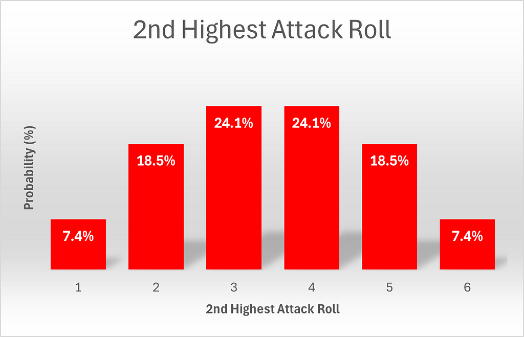
Note that the probabilities of attack results are exactly symmetrical. To be mathematically precise, P(x) = P(6-x). We will come back to this point.
We next compare the probabilities of attack and defense directly.
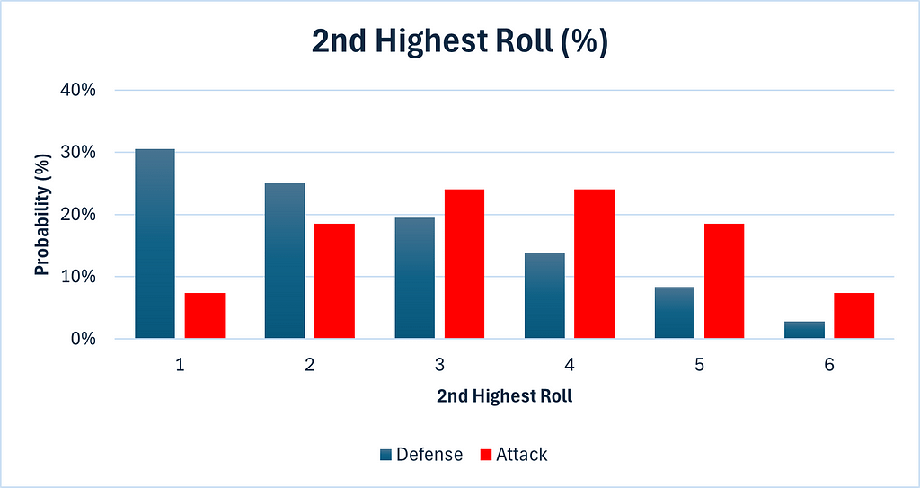
We can see that the attack has a significant advantage here. It is much more likely to obtain values of 4, 5 or 6, than defense is.
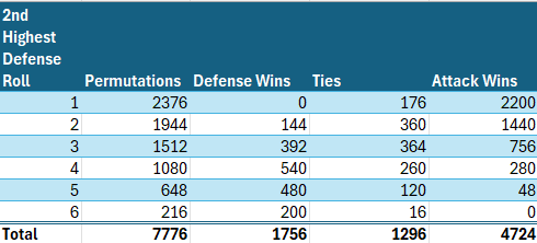
We are now ready to calculate the relative probabilities of victory for the second soldier. This segment is largely unchanged from the parallel calculations we did in Part 1. We need to count the permutations in which the defense achieves a 2nd highest roll of x, and then determine how many of those permutations yield an outright victory for the defense, a tie, or a win for the attack.
For example, since, as calculated above, there is a 3/36 chance of the defense’s second highest roll being 5, and there are a total of 6⁵= 7776 permutations, clearly (3/36) * 7776 = 648 of those permutations will yield a second highest defense roll of 5. To win, the attack then needs to get a second highest roll of 6, the probability of which is 16/216, as calculated above, so (16/216) * 648 = 48 of the 648 permutations which yielded a second highest defense roll of 5 will result in a victory for attack. To achieve a tie, attack must roll a 2nd highest roll of 5, the probability of which is 40/216, so (40/216) * 648 = 120 of those permutations will result in ties, and the remainder (648–120–48 = 480) will result in outright defense wins.
We can also calculate the respective conditional probabilities, in which we calculate the probabilities of victory for each team, given a particular defense roll.

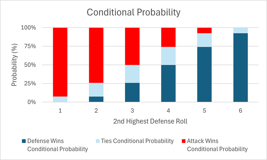
Note the exact symmetry of the above table and charts. Thus, the probabilities of an attack victory given a defense roll of x is identical to the probability of a defense victory given a defense roll of 6-x. Furthermore, the probability of a tie given a defense roll of x is identical to the probability of a tie given a defense roll of 6-x. This is of course because of the symmetry of the second highest roll of attack which was noted above.
As in Part 1, Table 4 and Chart 4 give a misleading impression. They imply that attack and defense are on an equal footing, but these are conditional probabilities and therefore they ignore how much more likely low rolls for defense are.
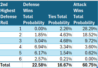
Total probabilities, on the other hand, will allow for this. In the table below, we see clearly that the attack will win from a defense roll of 1 significantly more often, in absolute terms, than defense will win from a defense roll of 6, despite the conditional symmetry noted above.
Below is a chart of total win probabilities by 2nd highest defensive roll.

The above chart finally captures what most of us felt instinctively, whether from experience of playing Risk or from mathematical instinct, that the attack has a big advantage. That advantage plays out specifically in the 2nd battle.
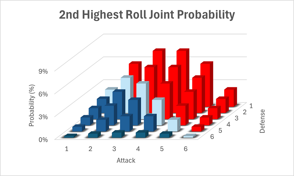
Finally, we can calculate the joint probability of each possible 2nd highest result for both attack and defense. A joint probability is simply the probability of two or more events co-occurring. Since the dice rolls of attack and defense are independent, the joint probability is simply the product of the individual probabilities of the respective rolls of attack and defense.

See the following graph for a cool visualization of the above chart. Note the configuration of the axes, which has been chosen to allow for best viewing.
There is one final factor we should consider, before we wrap up, and that is how likely it is for the attack to win both soldiers. However, compared to calculating the 3667 permutations and 4724 permutations which resulted in the attack winning the first and second soldiers respectively, which I calculated in my head (I had no choice, since I was asked the question on a religious holiday, on which I am forbidden to write, although admittedly I did have a choice about whether to brag about it), this calculation requires calculating and summing 36 separate permutation counts. This is because this calculation varies depending on both defense rolls simultaneously, while the previous calculations required considering the higher or lower roll of the defense independently. I will therefore not bore myself or you with calculating and summing all 36 permutation counts, and will rely on python to count the permutations. I will suffice with providing the code.
from itertools import product
import numpy as np
import pandas as pd


def check_both(result, attack_dice=3):
    """
    Given a result of multiple dice, and a number of attack dice, determine whether the attack will win both soldiers,
    the defense will both soldiers, or each will win a soldier.

    :param result: array of dice results, where the attack dice are declared first
    :param attack_dice: number of dice which represent the attack dice
    :return:
    """
    if np.partition(result[:attack_dice], -1)[-1] > np.partition(result[attack_dice:], -1)[-1] and
            np.partition(result[:attack_dice], -2)[-2] > np.partition(result[attack_dice:], -2)[-2]:
        return 'attack_both'
    elif np.partition(result[:attack_dice], -1)[-1] > np.partition(result[attack_dice:], -1)[-1] or
            np.partition(result[:attack_dice], -2)[-2] > np.partition(result[attack_dice:], -2)[-2]:
        return 'one_one'
    else:
        return 'defense_both'


# produce array of all possible permutations of 5 dice
arr = np.array(list(product([1, 2, 3, 4, 5, 6], [1, 2, 3, 4, 5, 6], [1, 2, 3, 4, 5, 6], [1, 2, 3, 4, 5, 6],
                            [1, 2, 3, 4, 5, 6]))).transpose()

# calculate and print counts of various result types
print(pd.Series(np.apply_along_axis(check_both, axis=0, arr=arr)).value_counts())
In the below graphics, a truce refers to a result where both attack and defense lose one soldier, while attack refers to the attack winning both soldiers and likewise for defense.

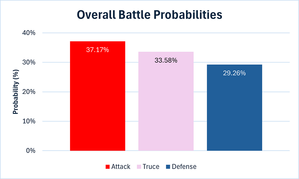
I thought for a second that I could finally use a pie chart for the above graphic without fear of criticism, but alas, the probabilities are too similar. The wait continues.
We can see that although the defense has a small advantage in the first battle, as we calculated in Part 1, the attack nevertheless has the upper hand overall, thanks to its significant advantage in the second battle.
Conclusions
- The probability of a victory for the attack is 60.75%. This can be seen clearly in Table 5.
- The probability of an outright victory for the defense is 22.58%. This can be seen clearly in Table 5.
- The probability of a tie is, perhaps a touch surprisingly, exactly 1/6, or 16.67%. This can be seen clearly in Table 5.
- If the defense’s second highest roll is 3, his probability of winning, including the probability of a tie, is exactly 50/50. This can be seen in Table 4.
- The probabilities of attack’s 2nd highest roll are exactly symmetrical. This can be seen in Table 2.
- The conditional probabilities are exactly symmetrical. This can be seen in Table 4.
- The most likely overall outcomes, at 7.36% each, are for the defense to roll a 1 and for the attack to roll either a 3 or a 4. This can be seen in Table 6.
- The probability of the attack winning both battles is 37.17%. This can be seen in Table 7.
- The probability of the defense winning both battles is 33.58%. This can be seen in Table 7.
- The probability of both the attack and defense winning a battle is 29.26%. This can be seen in Table 7.
We are now in a position to provide a definitive answer to our original question. The attack does have an overall advantage in a 3 to 2 dice battle.
I have to say I’ve enjoyed this foray into the mathematics and probability of Risk, and if you have too, well, that’s a bonus.
Until next time.
The Math Behind Risk — Part 2 was originally published in Towards Data Science on Medium, where people are continuing the conversation by highlighting and responding to this story.
Originally appeared here:
The Math Behind Risk — Part 2