The Math Behind KAN — Kolmogorov-Arnold Networks

The Math Behind KAN — Kolmogorov-Arnold Networks

A new alternative to the classic Multi-Layer Perceptron is out. Why is it more accurate and interpretable? Math and Code Deep Dive.

In today’s world of AI, neural networks drive countless innovations and advancements. At the heart of many breakthroughs is the Multi-Layer Perceptron (MLP), a type of neural network known for its ability to approximate complex functions. But as we push the boundaries of what AI can achieve, we must ask: Can we do better than the classic MLP?

Here’s Kolmogorov-Arnold Networks (KANs), a new approach to neural networks inspired by the Kolmogorov-Arnold representation theorem. Unlike traditional MLPs, which use fixed activation functions at each neuron, KANs use learnable activation functions on the edges (weights) of the network. This simple shift opens up new possibilities in accuracy, interpretability, and efficiency.

This article explores why KANs are a revolutionary advancement in neural network design. We’ll dive into their mathematical foundations, highlight the key differences from MLPs, and show how KANs can outperform traditional methods.

1: Limitations of MLPs

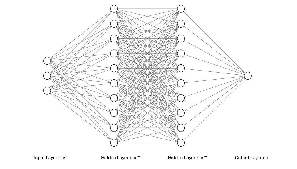
Multi-Layer Perceptrons (MLPs) are a core component of modern neural networks. They consist of layers of interconnected nodes, or “neurons,” designed to approximate complex, non-linear functions by learning from data. Each neuron uses a fixed activation function on the weighted sum of its inputs, transforming input data into the desired output through multiple layers of abstraction. MLPs have driven breakthroughs in various fields, from computer vision to speech recognition.

However, MLPs have some significant limitations:

1. Fixed Activation Functions on Nodes: Each node in an MLP has a predetermined activation function, like ReLU or Sigmoid. While effective in many cases, these fixed functions limit the network’s flexibility and adaptability. This can make it challenging for MLPs to optimize certain types of functions or adapt to specific data characteristics.
2. Interpretability Issues: MLPs are often criticized for being “black boxes.” As they become more complex, understanding their decision-making process becomes harder. The fixed activation functions and intricate weight matrices obscure the network’s inner workings, making it difficult to interpret and trust the model’s predictions without extensive analysis.

These drawbacks highlight the need for alternatives that offer greater flexibility and interpretability, paving the way for innovations like Kolmogorov-Arnold Networks (KANs).

2: Kolmogorov-Arnold Networks (KANs)

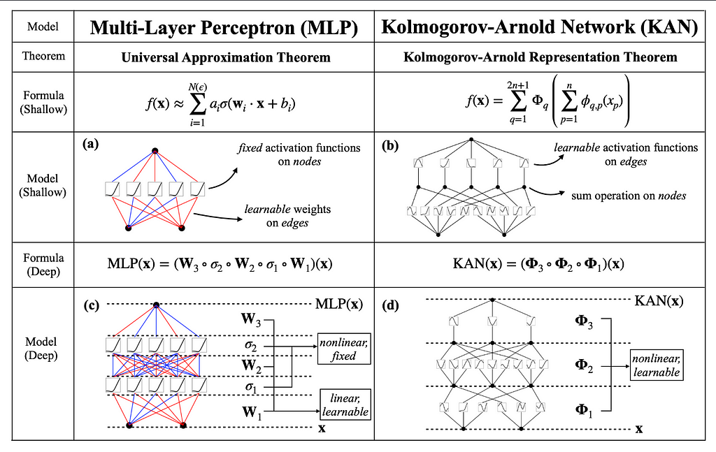
The Kolmogorov-Arnold representation theorem, formulated by mathematicians Andrey Kolmogorov and Vladimir Arnold, states that any multivariate continuous function can be represented as a finite composition of continuous functions of a single variable and the operation of addition. Think of this theorem as breaking down a complex recipe into individual, simple steps that anyone can follow. Instead of dealing with the entire recipe at once, you handle each step separately, making the overall process more manageable. This theorem implies that complex, high-dimensional functions can be broken down into simpler, univariate functions.

For neural networks, this insight is revolutionary, it suggests that a network could be designed to learn these univariate functions and their compositions, potentially improving both accuracy and interpretability.

KANs leverage the power of the Kolmogorov-Arnold theorem by fundamentally altering the structure of neural networks. Unlike traditional MLPs, where fixed activation functions are applied at each node, KANs place learnable activation functions on the edges (weights) of the network. This key difference means that instead of having a static set of activation functions, KANs adaptively learn the best functions to apply during training. Each edge in a KAN represents a univariate function parameterized as a spline, allowing for dynamic and fine-grained adjustments based on the data.

This change enhances the network’s flexibility and ability to capture complex patterns in data, providing a more interpretable and powerful alternative to traditional MLPs. By focusing on learnable activation functions on edges, KANs effectively utilize the Kolmogorov-Arnold theorem to transform neural network design, leading to improved performance in various AI tasks.

3: Mathematical Foundations

At the core of Kolmogorov-Arnold Networks (KANs) is a set of equations that define how these networks process and transform input data. The foundation of KANs lies in the Kolmogorov-Arnold representation theorem, which inspires the structure and learning process of the network.

Imagine you have an input vector x=[x1,x2,…,xn], which represents data points that you want to process. Think of this input vector as a list of ingredients for a recipe.

The theorem states that any complex recipe (high-dimensional function) can be broken down into simpler steps (univariate functions). For KANs, each ingredient (input value) is transformed through a series of simple steps (univariate functions) placed on the edges of the network. Mathematically, this can be represented as:

Here, ϕ_q,p​ are univariate functions that are learned during training. Think of ϕ_q,p​ as individual cooking techniques for each ingredient, and Φ_q as the final assembly step that combines these prepared ingredients.

Each layer of a KAN applies these cooking techniques to transform the ingredients further. For layer l, the transformation is given by:

Here, x(l) denotes the transformed ingredients at layer l, and ϕ_l,i,j are the learnable univariate functions on the edges between layer l and l+1. Think of this as applying different cooking techniques to the ingredients at each step to get intermediate dishes.

The output of a KAN is a composition of these layer transformations. Just as you would combine intermediate dishes to create a final meal, KANs combine the transformations to produce the final output:

Here, Φl represents the matrix of univariate functions at layer l. The overall function of the KAN is a composition of these layers, each refining the transformation further.

MLPs Structure
In traditional MLPs, each node applies a fixed activation function (like ReLU or sigmoid) to its inputs. Think of this as using the same cooking technique for all ingredients, regardless of their nature.

MLPs use linear transformations followed by these fixed non-linear activations:

where W represents the weight matrices, and σ represents the fixed activation functions.

Grid Extension Technique

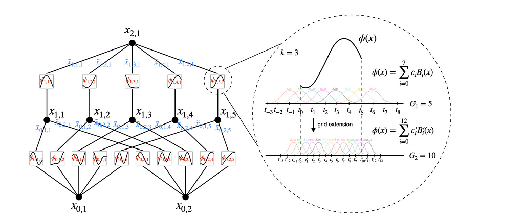
Grid extension is a powerful technique used to improve the accuracy of Kolmogorov-Arnold Networks (KANs) by refining the spline grids on which the univariate functions are defined. This process allows the network to learn increasingly detailed patterns in the data without requiring complete retraining.

These B-splines are a series of polynomial functions that are pieced together to form a smooth curve. They are used in KANs to represent the univariate functions on the edges. The spline is defined over a series of intervals called grid points. The more grid points there are, the finer the detail that the spline can capture

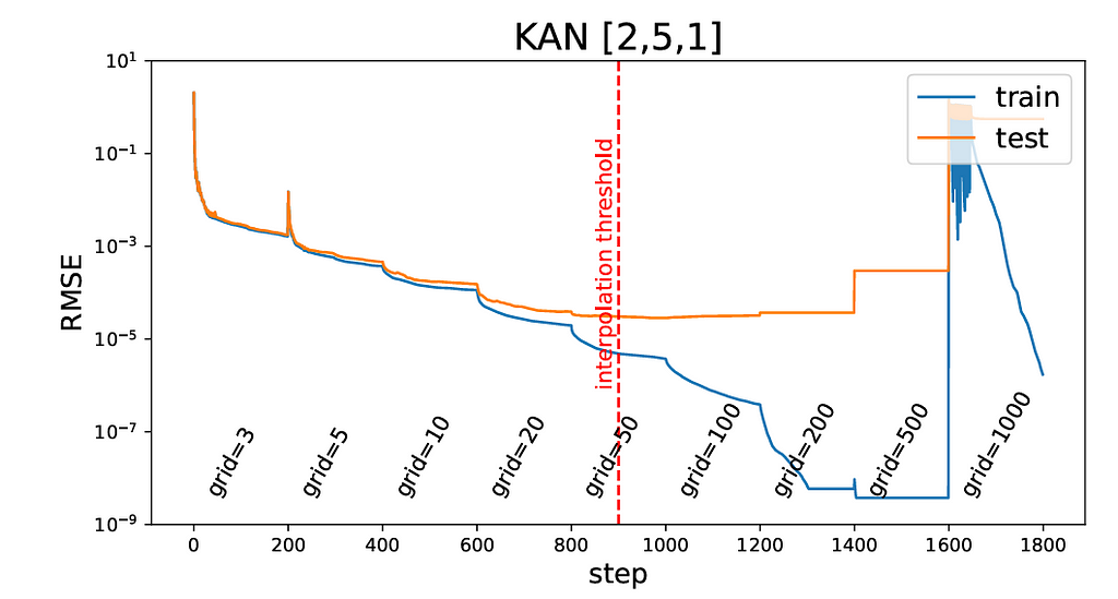
Initially, the network starts with a coarse grid, which means there are fewer intervals between grid points. This allows the network to learn the basic structure of the data without getting bogged down in details. Think of this like sketching a rough outline before filling in the fine details.

As training progresses, the number of grid points is gradually increased. This process is known as grid refinement. By adding more grid points, the spline becomes more detailed and can capture finer patterns in the data. This is similar to progressively adding more detail to your initial sketch, turning it into a detailed drawing.

Each increase introduces new B-spline basis functions B′_m​(x). The coefficients c’_m for these new basis functions are adjusted to ensure that the new, finer spline closely matches the original, coarser spline.

To achieve this match, least squares optimization is used. This method adjusts the coefficients c’_m​ to minimize the difference between the original spline and the refined spline.

Essentially, this process ensures that the refined spline continues to accurately represent the data patterns learned by the coarse spline.

Simplification Techniques

To enhance the interpretability of KANs, several simplification techniques can be employed, making the network easier to understand and visualize.

Sparsification and Pruning
This technique involves adding a penalty to the loss function based on the L1 norm of the activation functions. The L1 norm for a function ϕ is defined as the average magnitude of the function across all input samples:

Here, N_p​ is the number of input samples, and ϕ(x_s​) represents the value of the function ϕ for the input sample x_s​.

Think of sparsification like decluttering a room. By removing unnecessary items (or reducing the influence of less important functions), you make the space (or network) more organized and easier to navigate.

After applying L1 regularization, the L1 norms of the activation functions are evaluated. Neurons and edges with norms below a certain threshold are considered insignificant and are pruned away. The threshold for pruning is a hyperparameter that determines how aggressive the pruning should be.

Pruning is like trimming a tree. By cutting away the weak and unnecessary branches, you allow the tree to focus its resources on the stronger, more vital parts, leading to a healthier and more manageable structure.

Symbolification
Another approach is to replace learned univariate functions with known symbolic forms to make the network more interpretable.

The task is to identify potential symbolic forms (e.g., sin⁡, exp) that can approximate the learned functions. This step involves analyzing the learned functions and suggesting symbolic candidates based on their shape and behavior.

Once symbolic candidates are identified, use grid search and linear regression to fit parameters such that the symbolic function closely approximates the learned function.

4: KAN vs MLP in Python

To demonstrate the capabilities of Kolmogorov-Arnold Networks (KANs) compared to traditional Multi-Layer Perceptrons (MLPs), we will fit a function-generated dataset to both a KAN model and MLP model (leveraging PyTorch), to see what their performances look like.

The function we will be using is the same one used by the authors of the paper to show KAN’s capabilities vs MLP (Original paper example). However, the code will be different. You can find all the code we will cover today in this Notebook:

models-from-scratch-python/KAN – Kolmogorov-Arnold Networks/demo.ipynb at main · cristianleoo/models-from-scratch-python

Let’s import the required libraries, and generate the dataset

import numpy as np
import torch
import torch.nn as nn
from torchsummary import summary
from kan import KAN, create_dataset
import matplotlib.pyplot as plt

Here, we use:

• numpy: For numerical operations.
• torch: For PyTorch, which is used for building and training neural networks.
• torch.nn: For neural network modules in PyTorch.
• torchsummary: For summarizing the model structure.
• kan: Custom library containing the KAN model and dataset creation functions.
• matplotlib.pyplot: For plotting and visualizations.

# Define the dataset generation function
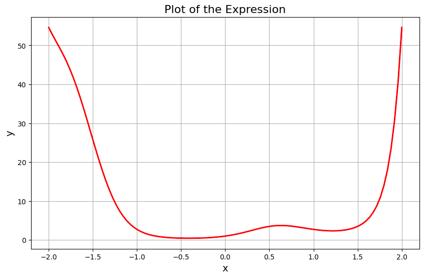
f = lambda x: torch.exp(torch.sin(torch.pi * x[:, [0]]) + x[:, [1]] ** 2)

This function includes both sinusoidal (sin) and exponential (exp) components. It takes a 2D input x and computes the output using the formula:

Let’s now fit a tensor of 100 points uniformly distributed between [-2, 2] to this function, to see what it looks like:

# Create the dataset
dataset = create_dataset(f, n_var=2)

create_dataset generates a dataset based on the function f. The dataset includes input-output pairs that will be used for training and testing the neural networks.

Now let’s build a KAN model and train it on the dataset.
We will start with a coarse grid (5 points) and gradually refine it (up to 100 points). This improves the model’s accuracy by capturing finer details in the data.

grids = np.array([5, 10, 20, 50, 100])
train_losses_kan = []
test_losses_kan = []
steps = 50
k = 3

for i in range(grids.shape[0]):
    if i == 0:
        model = KAN(width=[2, 1, 1], grid=grids[i], k=k)
    else:
        model = KAN(width=[2, 1, 1], grid=grids[i], k=k).initialize_from_another_model(model, dataset['train_input'])
    results = model.train(dataset, opt="LBFGS", steps=steps, stop_grid_update_step=30)
    train_losses_kan += results['train_loss']
    test_losses_kan += results['test_loss']

    print(f"Train RMSE: {results['train_loss'][-1]:.8f} | Test RMSE: {results['test_loss'][-1]:.8f}")

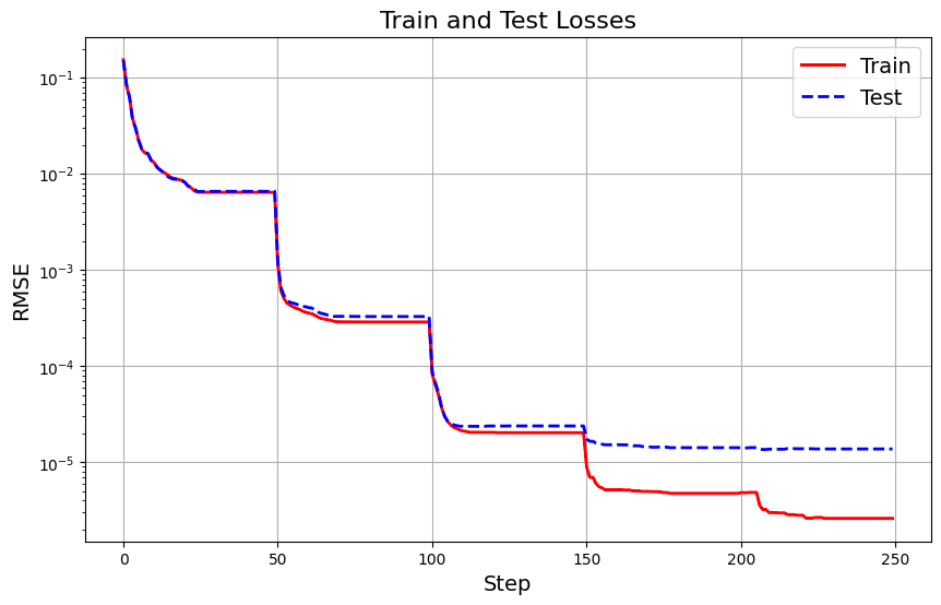
In this example, we define an array called grids with values [5, 10, 20, 50, 100]. We iterate over these grids to fit models sequentially, meaning each new model is initialized using the previous one.

For each iteration, we define a model with k=3, where k is the order of the B-spline. We set the number of training steps (or epochs) to 50. The model’s architecture consists of an input layer with 2 nodes, one hidden layer with 1 node, and an output layer with 1 node. We use the LFGBS optimizer for training.

Here are the training and test losses during the training process:

Let’s now define and train a traditional MLP for comparison.

# Define the MLP
class MLP(nn.Module):
    def __init__(self):
        super(MLP, self).__init__()
        self.layers = nn.Sequential(
            nn.Linear(dataset['train_input'].shape[1], 64),
            nn.ReLU(),
            nn.Linear(64, 64),
            nn.ReLU(),
            nn.Linear(64, 1)
        )
    def forward(self, x):
        return self.layers(x)

# Instantiate the model
model = MLP()
summary(model, input_size=(dataset['train_input'].shape[1],))

The MLP has an input layer, two hidden layers with 64 neurons each, and an output layer. ReLU activation is used between the layers.

criterion = nn.MSELoss()
optimizer = torch.optim.Adam(model.parameters(), lr=1e-2)
train_loss_mlp = []
test_loss_mlp = []

epochs = 250
for epoch in range(epochs):
    optimizer.zero_grad()
    output = model(dataset['train_input']).squeeze()
    loss = criterion(output, dataset['train_label'])
    loss.backward()
    optimizer.step()
    train_loss_mlp.append(loss.item()**0.5)

    # Test the model
    model.eval()
    with torch.no_grad():
        output = model(dataset['test_input']).squeeze()
        loss = criterion(output, dataset['test_label'])
        test_loss_mlp.append(loss.item()**0.5)

    print(f'Epoch {epoch+1}/{epochs}, Train Loss: {train_loss_mlp[-1]:.2f}, Test Loss: {test_loss_mlp[-1]:.2f}', end='r')

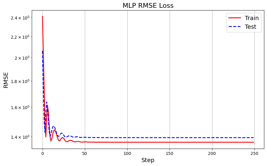
We use mean squared error (MSE) loss and Adam optimizer, and train the model for 250 epochs, recording the training and testing losses.

This is what the train and test RMSE look like in MLP:

Let’s put side to side the loss plots for a comparison:

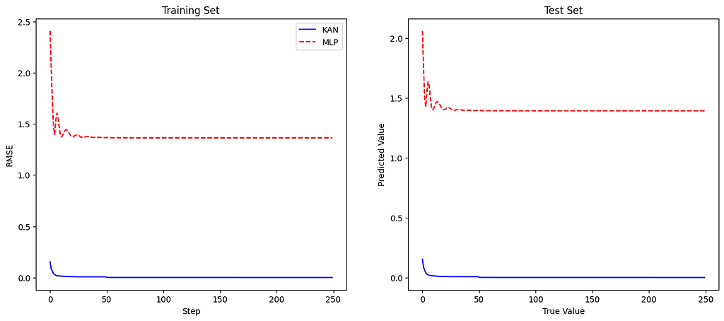
The plot shows that the KAN model achieves lower training RMSE than the MLP model, indicating better function-fitting capability. Similarly, the KAN model outperforms the MLP on the test set, demonstrating its superior generalization ability.

This example illustrates how KANs can more accurately fit complex functions than traditional MLPs, thanks to their flexible and adaptive structure. By refining the grid and employing learnable univariate functions on the edges, KANs capture intricate patterns in the data that MLPs may miss, leading to improved performance in function-fitting tasks.

Does this mean we should switch to KAN models permanently? Not necessarily.

KANs showed great results in this example, but when I tested them on other scenarios with real data, MLPs often performed better. One thing you’ll notice when working with KAN models is their sensitivity to hyperparameter optimization. Also, KANs have primarily been tested using spline functions, which work well for smoothly varying data like our example but might not perform as well in other situations.

In summary, KANs are definitely intriguing and have a lot of potential, but they need more study, especially regarding different datasets and the algorithm’s inner workings, to really make them work effectively.

5: Advantages of KANs

Accuracy

One of the standout advantages of Kolmogorov-Arnold Networks (KANs) is their ability to achieve higher accuracy with fewer parameters compared to traditional Multi-Layer Perceptrons (MLPs). This is primarily due to the learnable activation functions on the edges, which allow KANs to better capture complex patterns and relationships in the data.

Unlike MLPs that use fixed activation functions at each node, KANs use univariate functions on the edges, making the network more flexible and capable of fine-tuning its learning process to the data.

Because KANs can adjust the functions between layers dynamically, they can achieve comparable or even superior accuracy with a smaller number of parameters. This efficiency is particularly beneficial for tasks with limited data or computational resources.

Interpretability

KANs offer significant improvements in interpretability over traditional MLPs. This enhanced interpretability is crucial for applications where understanding the decision-making process is as important as the outcome.

KANs can be simplified through techniques like sparsification and pruning, which remove unnecessary functions and parameters. These techniques not only improve interpretability but also enhance the network’s performance by focusing on the most relevant components.

For some functions, it is possible to identify symbolic forms of the activation functions, making it easier to understand the mathematical transformations within the network.

Scalability

KANs exhibit faster neural scaling laws compared to MLPs, meaning they improve more rapidly as the number of parameters increases.

KANs benefit from more favorable scaling laws due to their ability to decompose complex functions into simpler, univariate functions. This allows them to achieve lower error rates with increasing model complexity more efficiently than MLPs.

KANs can start with a coarser grid and extend it to finer grids during training, which helps in balancing computational efficiency and accuracy. This approach allows KANs to scale up more gracefully than MLPs, which often require complete retraining when increasing model size.

Conclusion

Kolmogorov-Arnold Networks (KANs) present a groundbreaking alternative to traditional Multi-Layer Perceptrons (MLPs), offering several key innovations that address the limitations of their predecessors. By leveraging learnable activation functions on the edges rather than fixed functions at the nodes, KANs introduce a new level of flexibility and adaptability. This structural change leads to:

• Enhanced Accuracy: KANs achieve higher accuracy with fewer parameters, making them more efficient and effective for a wide range of tasks.
• Improved Interpretability: The ability to visualize and simplify KANs aids in understanding the decision-making process, which is crucial for critical applications in healthcare, finance, and autonomous systems.
• Better Scalability: KANs exhibit faster neural scaling laws, allowing them to handle increasing complexity more gracefully than MLPs.

The introduction of Kolmogorov-Arnold Networks marks an exciting development in the field of neural networks, opening up new possibilities for AI and machine learning.

References

• Ziming Liu, et al. “KAN: Kolmogorov-Arnold Networks”. https://arxiv.org/abs/2404.19756

The Math Behind KAN — Kolmogorov-Arnold Networks was originally published in Towards Data Science on Medium, where people are continuing the conversation by highlighting and responding to this story.