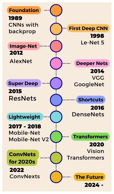
The History of Convolutional Neural Networks for Image Classification (1989 – Today)
A visual tour of the greatest innovations in Deep Learning and Computer Vision.
Before CNNs, the standard way to train a neural network to classify images was to flatten it into a list of pixels and pass it through a feed-forward neural network to output the image’s class. The problem with flattening the image is that the essential spatial information in the image is discarded.
In 1989, Yann LeCun and team introduced Convolutional Neural Networks — the backbone of Computer Vision research for the last 15 years! Unlike feedforward networks, CNNs preserve the 2D nature of images and are capable of processing information spatially!
In this article, we are going to go through the history of CNNs specifically for Image Classification tasks — starting from those early research years in the 90’s to the golden era of the mid-2010s when many of the most genius Deep Learning architectures ever were conceived, and finally discuss the latest trends in CNN research now as they compete with attention and vision-transformers.
Check out the YouTube video that explains all the concepts in this article visually with animations. Unless otherwise specified, all the images and illustrations used in this article are generated by myself during creating the video version.

The Basics of Convolutional Neural Networks
At the heart of a CNN is the convolution operation. We scan the filter across the image and calculate the dot product of the filter with the image at each overlapping location. This resulting output is called a feature map and it captures how much and where the filter pattern is present in the image.
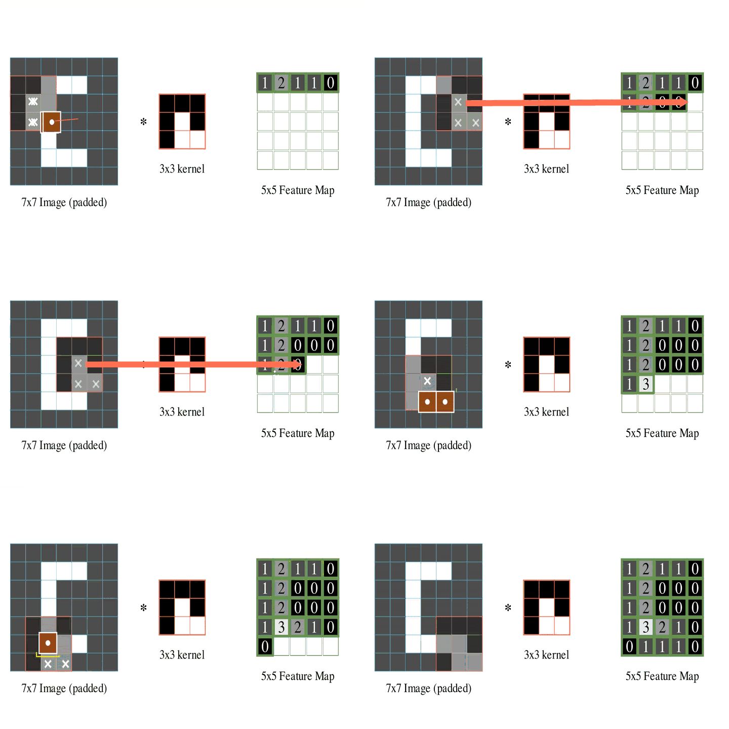
In a convolution layer, we train multiple filters that extract different feature maps from the input image. When we stack multiple convolutional layers in sequence with some non-linearity, we get a convolutional neural network (CNN).
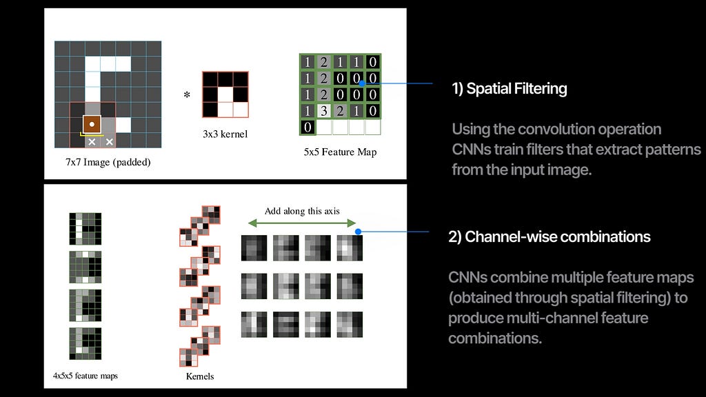
So each convolution layer simultaneously does 2 things —
1. spatial filtering with the convolution operation between images and kernels, and
2. combining the multiple input channels and output a new set of channels.
90 percent of the research in CNNs has been to modify or to improve just these two things.
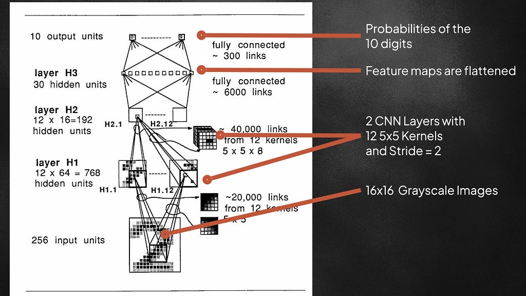
The 1989 Paper
This 1989 paper taught us how to train non-linear CNNs from scratch using backpropagation. They input 16×16 grayscale images of handwritten digits, and pass through two convolutional layers with 12 filters of size 5×5. The filters also move with a stride of 2 during scanning. Strided-convolution is useful for downsampling the input image. After the conv layers, the output maps are flattened and passed through two fully connected networks to output the probabilities for the 10 digits. Using the softmax cross-entropy loss, the network is optimized to predict the correct labels for the handwritten digits. After each layer, the tanh nonlinearity is also used — allowing the learned feature maps to be more complex and expressive. With just 9760 parameters, this was a very small network compared to today’s networks which contain hundreds of millions of parameters.
Inductive Bias
Inductive Bias is a concept in Machine Learning where we deliberately introduce specific rules and limitations into the learning process to move our models away from generalizations and steer more toward solutions that follow our human-like understanding.
When humans classify images, we also do spatial filtering to look for common patterns to form multiple representations and then combine them together to form our predictions. The CNN architecture is designed to replicate just that. In feedforward networks, each pixel is treated like it’s own isolated feature as each neuron in the layers connects with all the pixels — in CNNs there is more parameter-sharing because the same filter scans the entire image. Inductive biases make CNNs less data-hungry too because they get local pattern recognition for free due to the network design but feedforward networks need to spend their training cycles learning about it from scratch.
Le-Net 5 (1998)

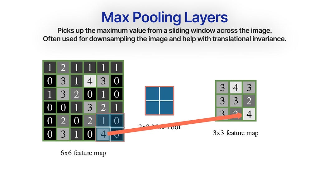
In 1998, Yann LeCun and team published the Le-Net 5 — a deeper and larger 7-layer CNN model network. They also use Max Pooling which downsamples the image by grabbing the maximum values from a 2×2 sliding window.
Local Receptive Field
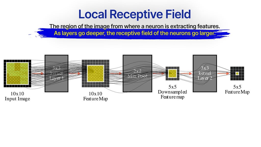
Notice when you train a 3×3 conv layer, each neuron is connected to a 3×3 region in the original image — this is the neuron’s local receptive field — the region of the image where this neuron extracts patterns from.
When we pass this feature map through another 3×3 layer , the new feature map indirectly creates a receptive field of a larger 5×5 region from the original image. Additionally, when we downsample the image through max-pooling or strided-convolution, the receptive field also increases — making deeper layers access the input image more and more globally.
For this reason, earlier layers in a CNN can only pick low-level details like specific edges or corners, and the latter layers pick up more spread-out global-level patterns.
The Draught (1998–2012)
As impressive Le-Net-5 was, researchers in the early 2000s still deemed neural networks to be computationally very expensive and data hungry to train. There was also problems with overfitting — where a complex neural network will just memorize the entire training dataset and fail to generalize on new unseen datasets. The researchers instead focused on traditional machine learning algorithms like support vector machines that were showing much better performance on the smaller datasets of the time with much less computational demands.
ImageNet Dataset (2009)
The ImageNet dataset was open-sourced in 2009 — it contained 3.2 million annotated images at the time covering over 1000 different classes. Today it has over 14 million images and over 20,000 annotated different classes. Every year from 2010 to 2017 we got this massive competition called the ILSVRC where different research groups will publish models to beat the benchmarks on a subset of the ImageNet dataset. In 2010 and 2011, traditional ML methods like Support Vector Machines were winning — but starting from 2012 it was all about CNNs. The metric used to rank different networks was generally the top-5 error rate — measuring the percentage of times that the true class label was not in the top 5 classes predicted by the network.
AlexNet (2012)
AlexNet, introduced by Dr. Geoffrey Hinton and his team was the winner of ILSVRC 2012 with a top-5 test set error of 17%. Here are the three main contributions from AlexNet.
1. Multi-scaled Kernels
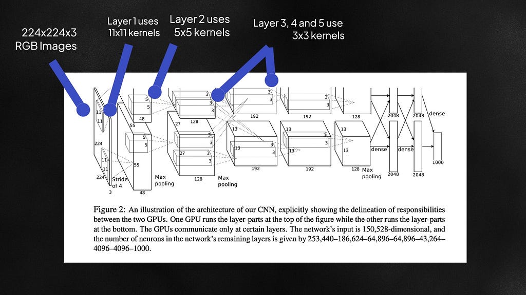
AlexNet trained on 224×224 RGB images and used multiple kernel sizes in the network — an 11×11, a 5×5, and a 3×3 kernel. Models like Le-Net 5 only used 5×5 kernels. Larger kernels are more computationally expensive because they train more weights, but also capture more global patterns from the image. Because of these large kernels, AlexNet had over 60 million trainable parameters. All that complexity can however lead to overfitting.
2. Dropout
To alleviate overfitting, AlexNet used a regularization technique called Dropout. During training, a fraction of the neurons in each layer is turned to zero. This prevents the network from being too reliant on specific neurons or groups of neurons for generating a prediction and instead encourages all the neurons to learn general meaningful features useful for classification.
3. RELU
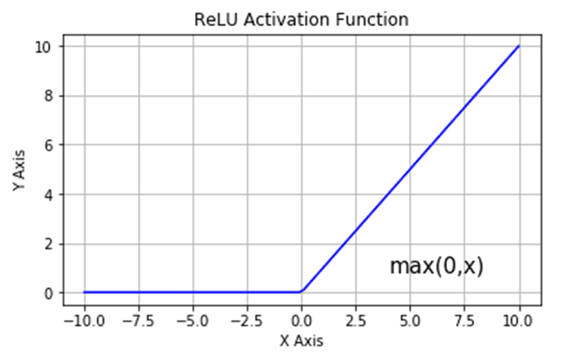
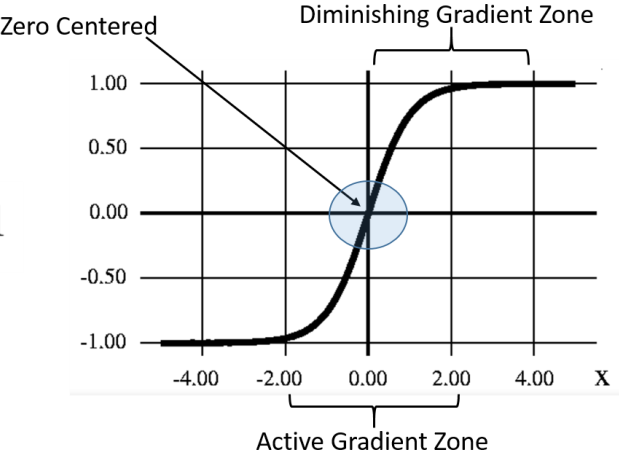
Alexnet also replaced tanh nonlinearity with ReLU. RELU is an activation function that turns negative values to zero and keeps positive values as-is. The tanh function tends to saturate for deep networks because the gradients get low when the value of x goes too high or too low making optimization slow. RELU offers a steady gradient signal to train the network about 6 times faster than tanH.

AlexNet also introduced the concept of Local Response Normalization and strategies for distributed CNN training.
GoogleNet / Inception (2014)
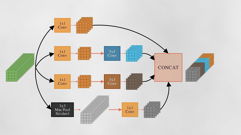
In 2014, GoogleNet paper got an ImageNet top-5 error rate of 6.67%. The core component of GoogLeNet was the inception module. Each inception module consists of parallel convolutional layers with different filter sizes (1×1, 3×3, 5×5) and max-pooling layers. Inception applies these kernels to the same input and then concats them, combining both low-level and medium-level features.
1×1 Convolution
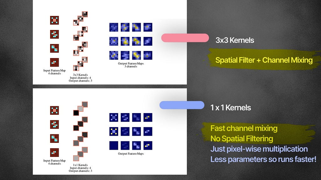
They also use 1×1 convolutional layer. Each 1×1 kernel first scales the input channels and then combines them. 1×1 kernels multiply each pixel with a fixed value — which is why it is also called pointwise convolutions.
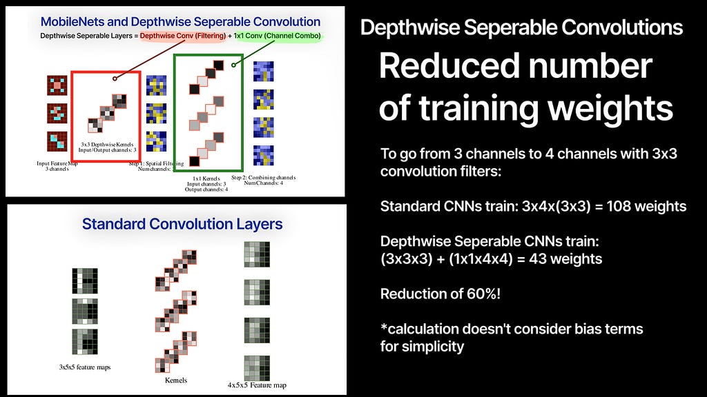
While larger kernels like 3×3 and 5×5 kernels do both spatial filtering and channel combination, 1×1 kernels are only good for channel mixing, and it does so very efficiently with a lower number of weights. For example, A 3-by-4 grid of 1×1 convolution layers trains only (1×1 x 3×4 =) 12 weights — but if it were 3×3 kernels — we would train (3×3 x 3×4 =) 108 weights.
Dimensionality Reduction
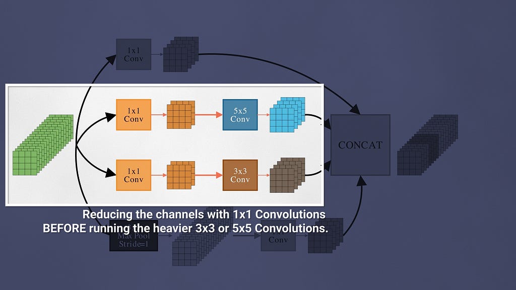
GoogleNet uses 1×1 conv layers as a dimensionality reduction method to reduce the number of channels before running spatial filtering with the 3×3 and 5×5 convolutions on these lower dimensional feature maps. This helps them to cut down on the number of trainable weights compared to AlexNet.
VGGNet (2014)
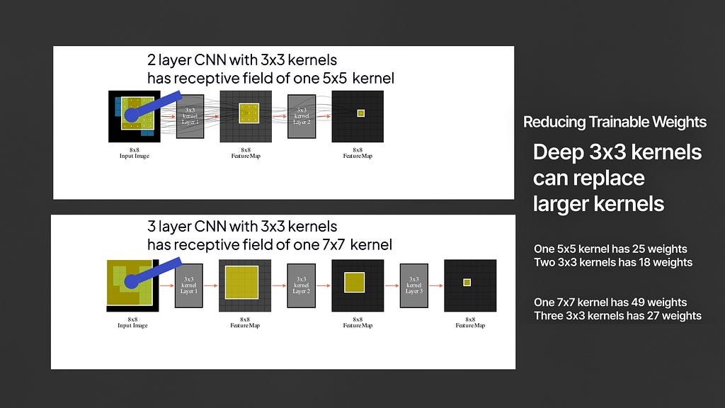
The VGG Network claims that we do not need larger kernels like 5×5 or 7×7 networks and all we need are 3×3 kernels. 2 layer 3×3 convolutional layer has the same receptive field of the image that a single 5×5 layer does. Three 3×3 layers have the same receptive field that a single 7×7 layer does.
Deep 3×3 Convolution Layers capture the same receptive field as larger kernels but with fewer parameters!
One 5×5 filter trains 25 weights — while two 3×3 filters train 18 weights. Similarly one 7×7 trains 49 weights, while 3 3×3 trains just 27. Training with deep 3×3 convolution layers became the standard for a long time in CNN architectures.
Batch Normalization (2015)
Deep neural networks can suffer from a problem known as “Internal Covariate Shift” during training. Since the earlier layers of the network are constantly training, the latter layers need to continuously adapt to the constantly shifting input distribution it receive from the previous layers.
Batch Normalization aims to counteract this problem by normalizing the inputs of each layer to have zero mean and unit standard deviation during training. A batch normalization or BN layer can be applied after any convolution layer. During training it subtracts the mean of the feature map along the minibatch dimension and divides it by the standard deviation. This means that each layer will now see a more stationary unit gaussian distribution during training.
Advantages of Batch Norm
- converge around 14 times faster
- let us use higher learning rates, and
- makes the network robust to the initial weights of the network.
ResNets (2016)
Deep Networks struggle to do Identity Mapping
Imagine you have a shallow neural network that has great accuracy on a classification task. Turns out that if we added 100 new convolution layers on top of this network, the training accuracy of the model could go down!
This is quite counter-intuitive because all these new layers need to do is copy the output of the shallow network at each layer — and at least be able to match the original accuracy. In reality, deep networks can be notoriously difficult to train because gradients can saturate or become unstable when backpropagating through many layers. With Relu and batch norm, we were able to train 22-layer deep CNNs at this point — the good folks at Microsoft introduced ResNets in 2015 which allowed us to stably train 150 layered CNNs. What did they do?
Residual learning
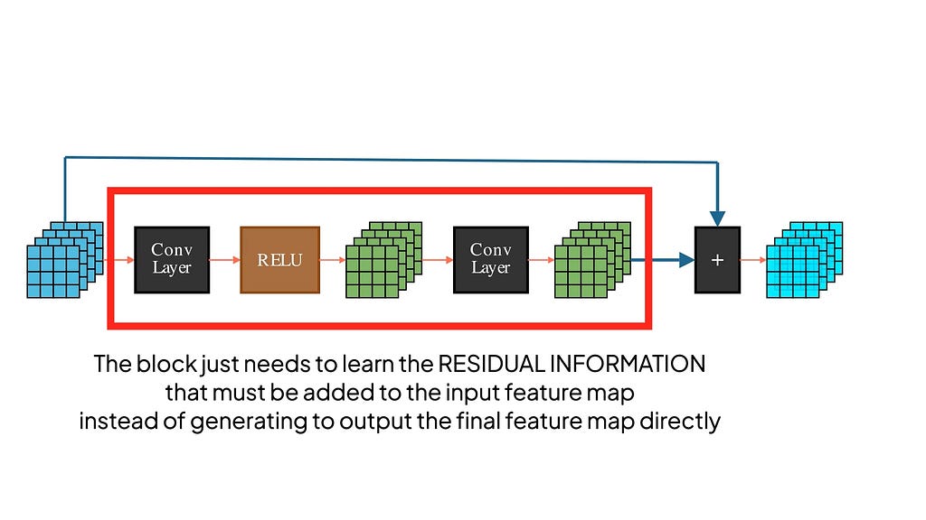
The input passes through one or more CNN layers as usual, but at the end, the original input is added back to the final output. These blocks are called residual blocks because they don’t need to learn the final output feature maps in the traditional sense — but they are just the residual features that must be added to the input to get the final feature maps. If the weights in the middle layers were to turn themselves to ZERO, then the residual block would just return the identity function — meaning it would be able to easily copy the input X.
Easy Gradient Flow
During backpropagation gradients can directly flow through these shortcut paths to reach the earlier layers of the model faster, helping to prevent gradient vanishing issues. ResNet stacks many of these blocks together to form really deep networks without any loss of accuracy!
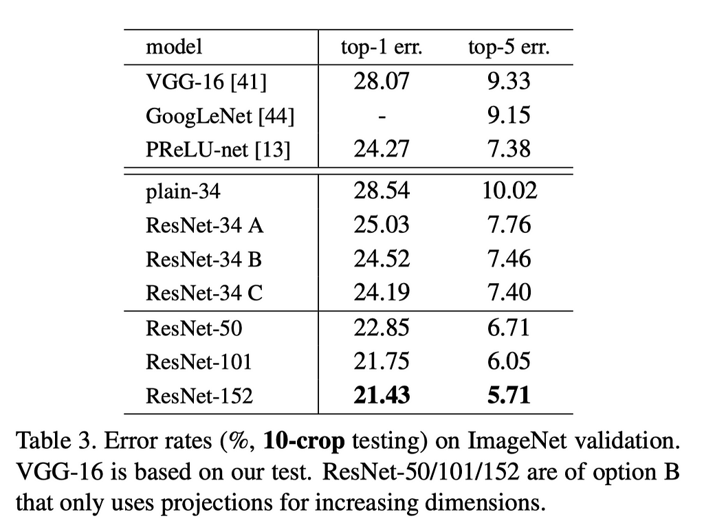
And with this remarkable improvement, ResNets managed to train a 152-layered model that got a top-5 error rate that shattered all previous records!
DenseNet (2017)
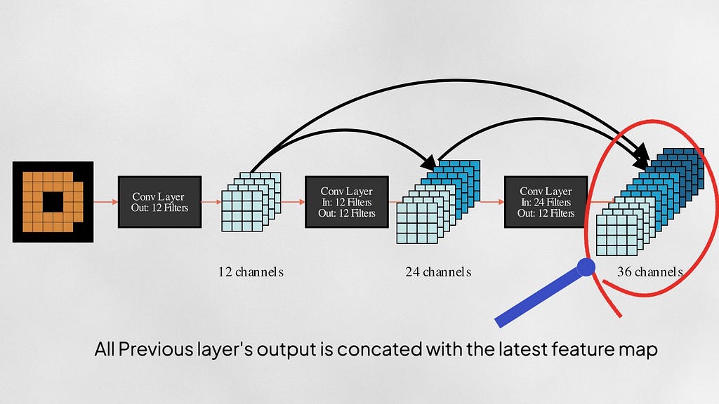
Dense-Nets also add shortcut paths connecting earlier layers with the latter layers in the network. A DenseNet block trains a series of convolution layers, and the output of every layer is concatenated with the feature maps of every previous layer in the block before passing to the next layer. Each layer adds only a small number of new feature maps to the “collective knowledge” of the network as the image flows through the network. DenseNets have an improved flow of information and gradients throughout the network because each layer has direct access to the gradients from the loss function.
Squeeze and Excitation Network (2017)
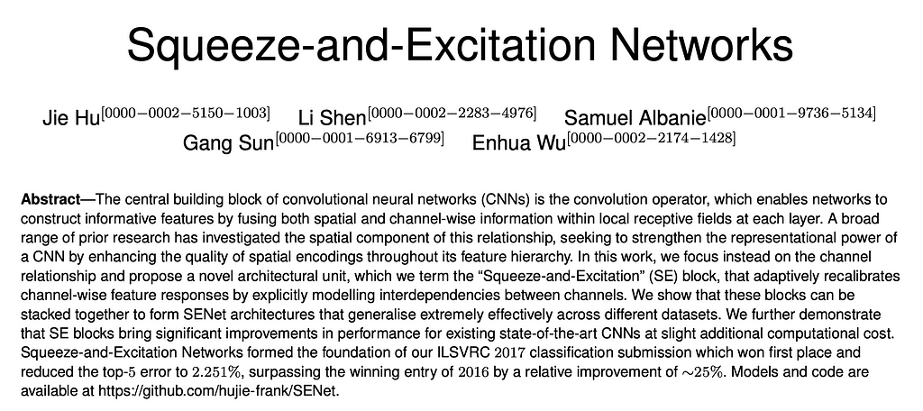
SEN-NET was the final winner of the ILSVRC competition, which introduced the Squeeze and Excitation Layer into CNNs. The SE block is designed to explicitly model the dependencies between all the channels of a feature map. In normal CNNs, each channel of a feature map is computed independently of each other; SEN-Net applies a self-attention-like method to make each channel of a feature map contextually aware of the global properties of the input image. SEN-Net won the final ILVSRC of 2017, and one of the 154-layered SenNet + ResNet models got a ridiculous top-5 error rate of 4.47%.
Squeeze Operation
The squeeze operation compresses the spatial dimensions of the input feature map into a channel descriptor using global average pooling. Since each channel contains neurons that capture local properties of the image, the squeeze operation accumulates global information about each channel.
Excitation Operation
The excitation operation rescales the input feature maps by channel-wise multiplication with the channel descriptors obtained from the squeeze operation. This effectively propagates global-level information to each channel — contextualizing each channel with the rest of the channels in the feature map.

MobileNet (2017)
Convolution layers do two things –1) filtering spatial information and 2) combining them channel-wise. The MobileNet paper uses Depthwise Separable Convolution, a technique that separates these two operations into two different layers — Depthwise Convolution for filtering and pointwise convolution for channel combination.
Depthwise Convolution
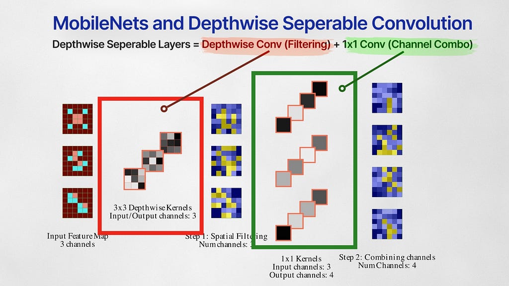
Given an input set of feature maps with M channels, first, they use depthwise convolution layers that train M 3×3 convolutional kernels. Unlike normal convolution layers that perform convolution on all feature maps, depthwise convolution layers train filters that perform convolution on just one feature map each. Secondly, they use 1×1 pointwise convolution filters to mix all these feature maps. Separating the filtering and combining steps like this drastically reduces the number of weights, making it super lightweight while still retaining the performance.
MobileNetV2 (2019)
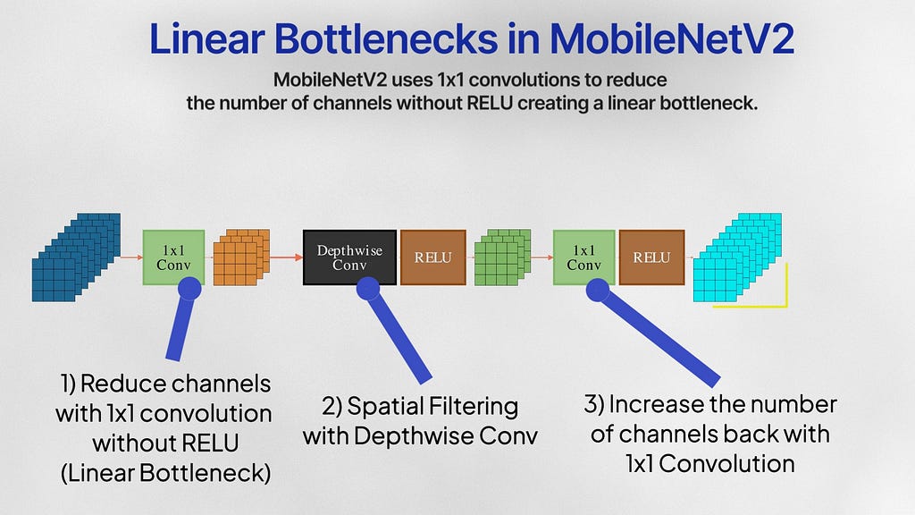
In 2018, MobileNetV2 improved the MobileNet architecture by introducing two more innovations: Linear Bottlenecks and Inverted residuals.
Linear Bottlenecks
MobileNetV2 uses 1×1 pointwise convolution for dimensionality reduction, followed by depthwise convolution layers for spatial filtering, and another 1×1 pointwise convolution layer to expand the channels back. These bottlenecks don’t pass through RELU and are instead kept linear. RELU zeros out all the negative values that came out of the dimensionality reduction step — and this can cause the network to lose valuable information especially if a bulk of this lower dimensional subspace was negative. Linear layers prevent the loss of excessive information during this bottleneck.
Inverted Residuals
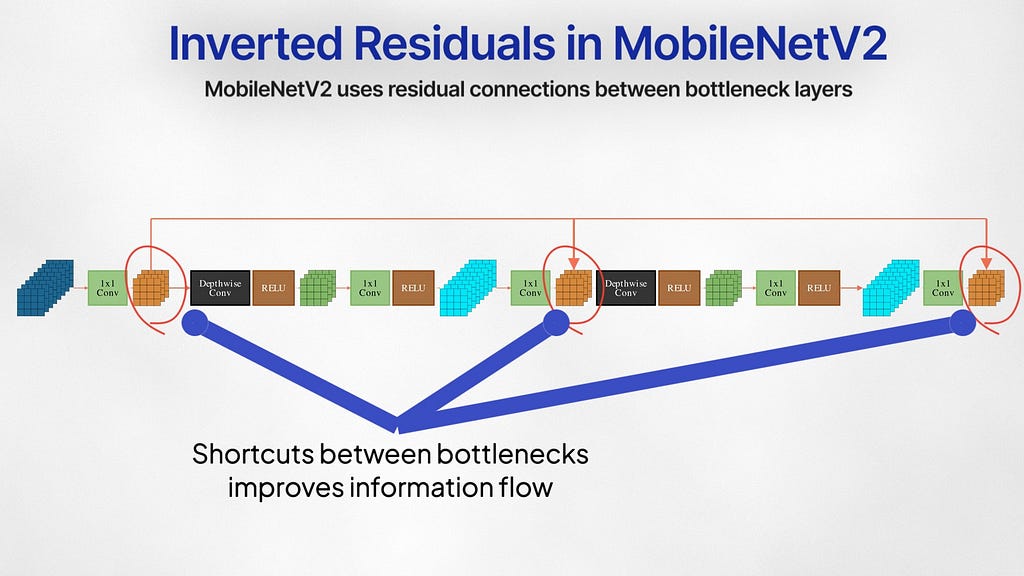
The second innovation is called Inverted Residuals. Generally, residual connections occur between layers with the highest channels, but the authors add shortcuts between the bottlenecks layers. The bottleneck captures the relevant information within a low-dimensional latent space, and the free flow of information and gradient between these layers is the most crucial.
Vision Transformers (2020)
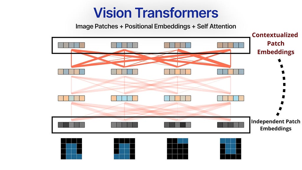
Vision Transformers or ViTs established that transformers can indeed beat state-of-the-art CNNs in Image Classification. Transformers and Attention mechanisms provide a highly parallelizable, scalable, and general architecture for modeling sequences. Neural Attention is a whole different area of Deep Learning, which we won’t get into this article, but feel free to learn more in this Youtube video.
ViTs use Patch Embeddings and Self-Attention
The input image is first divided into a sequence of fixed-size patches. Each patch is independently embedded into a fixed-size vector either through a CNN or passing through a linear layer. These patch embeddings and their positional encodings are then inputted as a sequence of tokens into a self-attention-based transformer encoder. Self-attention models the relationships between all the patches, and outputs new updated patch embeddings that are contextually aware of the entire image.
Inductive Bias vs Generality
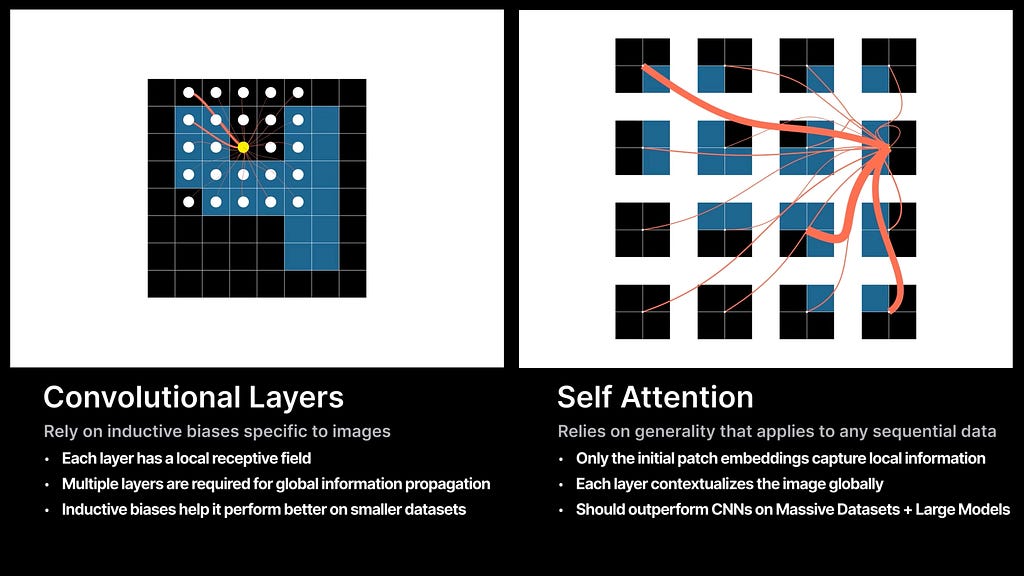
Where CNNs introduce several inductive biases about images, Transformers do the opposite — No localization, no sliding kernels — they rely on generality and raw computing to model the relationships between all the patches of the image. The Self-Attention layers allow global connectivity between all patches of the image irrespective of how far they are spatially. Inductive biases are great on smaller datasets, but the promise of Transformers is on massive training datasets, a general framework is going to eventually beat out the inductive biases offered by CNNs.
ConvNext — A ConvNet for the 2020s (2022)
A great choice to include in this article would be Swin Transformers, but that is a topic for a different day! Since this is a CNN article, let’s focus on one last CNN paper.
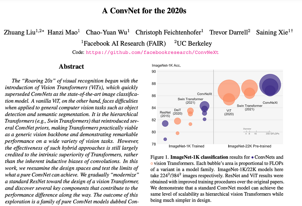
Patchifying Images like VITs
The input of ConvNext follows the patching strategy inspired by Vision Transformers. A 4×4 convolution kernel with a stride of 4 creates a downsampled image which is inputted into the rest of the network.
Depthwise Separable Convolution
Inspired by MobileNet, ConvNext uses depthwise separable convolution layers. The authors also hypothesize depthwise convolution is similar to the weighted sum operation in self-attention, which operates on a per-channel basis by only mixing information in the spatial dimension. Also the 1×1 pointwise convolutions are similar to the channel mixing steps in Self-Attention.
Larger Kernel Sizes
While ConvNets have been using 3×3 kernels ever since VGG, ConvNext proposes larger 7×7 filters to capture a wider spatial context, trying to come close to the fully global context that ViTs capture, while retaining the localization spirits of CNNs.
There are also some other tweaks, like using MobileNetV2-inspired inverted bottlenecks, the GELU activations, layer norms instead of batch norms, and more that shape up the rest of the ConvNext architecture.
Scalability
ConvNext are more computationally efficient way with the depthwise separable convolutions and is more scalable than transformers on high-resolution images — this is because Self-Attention scales quadratically with sequence length and Convolution doesn’t.

Final Thoughts!
The history of CNNs teaches us so much about Deep Learning, Inductive Bias, and the nature of computation itself. It’ll be interesting to see what wins out in the end — the inductive biases of ConvNets or the Generality of Transformers. Do check out the companion YouTube video for a visual tour of this article, and the individual papers as listed below.
References
CNN with Backprop (1989): http://yann.lecun.com/exdb/publis/pdf/lecun-89e.pdf
LeNet-5: http://vision.stanford.edu/cs598_spring07/papers/Lecun98.pdf
GoogleNet: https://arxiv.org/abs/1409.4842
VGG: https://arxiv.org/abs/1409.1556
Batch Norm: https://arxiv.org/pdf/1502.03167
ResNet: https://arxiv.org/abs/1512.03385
DenseNet: https://arxiv.org/abs/1608.06993
MobileNet: https://arxiv.org/abs/1704.04861
MobileNet-V2: https://arxiv.org/abs/1801.04381
Vision Transformers: https://arxiv.org/abs/2010.11929
ConvNext: https://arxiv.org/abs/2201.03545
Squeeze-and-Excitation Network: https://arxiv.org/abs/1709.01507
Swin Transformers: https://arxiv.org/abs/2103.14030
The History of Convolutional Neural Networks for Image Classification (1989- Today) was originally published in Towards Data Science on Medium, where people are continuing the conversation by highlighting and responding to this story.
Originally appeared here:
The History of Convolutional Neural Networks for Image Classification (1989- Today)
