
Continue the journey for evolving networks
Many complex networks evolve over time including transaction networks, traffic networks, social networks and more. Temporal Graph Learning (TGL) is a fast growing field which aims to learn, predict and understand evolving networks. See our previous blog post for an introduction to temporal graph learning and a summary of advancements last year.
In 2023, we saw significantly increased interest from both academia and the industry in the development of TGL. Compared to last year, the number of submissions at the temporal graph learning workshop @ NeurIPS 2023 tripled, resulting in 35 accepted papers. In addition, the temporal graph learning reading group, started in February 2023, has now hosted 28 research talks (find the recordings on YouTube). With nearly 200 researchers signed up for the reading group, we are glad to see witness interest in the topic and an extremely active community.

This post was co-authored with Emanuele Rossi, Michael Galkin ,Andrea Cini and Ingo Scholtes.
This blog post covers a selection of exciting developments in TGL while pointing out research directions for 2024. We also ask leading researchers for their take on what the future holds for TGL. This blog also aims to provide references and act as starting points for those who want to learn more about temporal graph learning. Please share with us in the comment section any other advances you are excited about.
Table of Contents:
- Temporal Graph Benchmark
- Novel Architectures for Link Prediction
- Spatiotemporal Graphs and Graph Deep Learning for Time Series Processing
- Temporal Knowledge Graph
- Causality-Aware Temporal Graph Learning
- Explainable Temporal Graph Methods
- Adversarial Attacks on Temporal Graphs
- Libraries and Benchmarks
- Joining Temporal Graph Learning Community
Temporal Graph Benchmark
One of the driving forces of the rapid development of machine learning on graphs is the availability of standardized and diverse benchmarks such as the Open Graph Benchmark (OGB), the Long Range Graph Benchmark and GraphWorld. However, these benchmarks are designed for static graphs and lack the fine-grained timestamp information required for temporal graph learning. Therefore, progress in temporal graph learning has been held back by the lack of large high-quality datasets, as well as the lack of proper evaluation resulting in over-optimistic performances.
To address this gap, the Temporal Graph Benchmark (TGB) was presented recently, including a collection of challenging and diverse benchmark datasets for realistic, reproducible, and robust evaluation for machine learning on temporal graphs. TGB provides a pypi package to automatically download and process nine datasets from five distinct domains with up to 72 million edges and 30 million timestamps. TGB also provides standardized evaluation motivated by real applications.
Image source: Huang et al. 2023, by authors.
TGB includes both link and node level tasks and an extensive empirical comparison of state-of-the-art TG models on all datasets. The first task is the dynamic link property prediction task which predicts the property (often existence) of a link between a pair of nodes at a future time. In TGB, this task is modeled as a ranking problem and evaluated with the filtered Mean Reciprocal Rank (MRR) metric. Results show that model rankings vary significantly across datasets with different ratios of test set edges which are never observed during training. In addition, model performance deteriorates as more negative samples (non-existence edges) are used in the evaluation. Interestingly, the extent of performance drop varies across models as well.
In the dynamic node property prediction task, the goal is to predict the property of a node at a given time. More specifically we focus on the node affinity prediction task which models how the user preference towards different items shift over time. Here, we use the Normalized Discounted Cumulative Gain of the top 10 items (NDCG@10) to compare the relative order of the predicted items to that of the ground truth. Interesting, we found that single heuristics outperform existing TG models and this highlights the need for more models focusing on node level tasks in the future. The TGB leaderboard is public and you are welcome to submit your model via a google form. For more details, see the TGB blog post by the authors of this blog.
Novel Architectures for Link Prediction
“Link prediction in the realm of temporal graph learning poses a significant challenge. The learning algorithms must extend beyond the limited expressive power typically found in traditional message passing architectures like GNNs. Additionally, they must emphasize computational efficiency. A critical aspect of this is ensuring low latency in responding to link prediction queries, striking a balance between the expressive power of the model and the speed of its predictions in a dynamic and complex data environment.” — Pan Li, Assistant Professor, Georgia Institute of Technology
A recent survey by Longa et al. provides a comprehensive overview of temporal GNNs. Many approaches proposed specialized architectures for dynamic link prediction, often aiming to capture important structure properties or correlations. For example, Luo et al. aimed to explicitly model the joint neighborhood of a set of nodes for future link prediction where they designed the Neighborhood-Aware Temporal network model (NAT). The joint neighborhood is not captured by traditional Graph Neural Network (GNN) based approaches as the node embedding vectors are generated independently for each node. In the following example, node v and w have the same structural contexts thus indistinguishable in the eyes of GNNs. In reality, the link between node u and v at t₃ is more likely to form due to the triadic closure law while this is not sure for the link between u and w at t₃. In comparison, NAT adapted a novel dictionary-type neighborhood representation which records k-hop neighborhood information and allows fast construction of structure features of joint neighborhood of multiple nodes. The dictionary representation is maintained by an efficient cache technique named N-cache. N-caches allowed NAT to construct the joint neighborhood features for a batch of node pairs for fast link prediction.
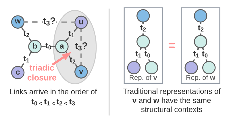
Image source: Luo et al. 2022
Second, Yu et al. aim to capture long-term temporal dependencies by proposing DyGFormer, a new Transformer-based architecture for temporal graph learning. Given a query between node u and node v at time t, the first step is to extract historical first-hop interactions of node u and v before time t. This includes the encodings of neighbors, links, time intervals as well as the frequencies of every neighbor’s appearances of u and v. The assumption is that if u and v share more common historical neighbors in the past, then they are more likely to interact in the future. After encoding the historical interactions in a sequence, it is then divided into multiple patches and fed into a transformer for capturing temporal dependencies.
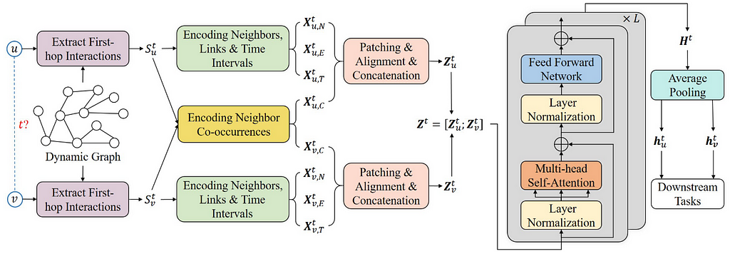
Image source: Yu et al. 2023
Another question is do we really need complicated model architectures for temporal networks? In a paper with the same name, Cong et al. examined the necessity of common modules used in temporal graph learning such as Recurrent Neural Network (RNN) and the self-attention mechanism. They showed that these modules are not always necessary for dynamic link prediction. In particular, their proposed GraphMixer model is based entirely on multi-layer perceptrons (MLPs) and neighbor mean-pooling while performing strongly against baselines with RNN and self-attention. GraphMixer contains three modules: a link-encoder summarizes the information from temporal links, a node-encoder extracts information from nodes and a link-classifier which combines the above information for prediction. Interestingly, Cong et al. argued that a trainable time-encoding function could cause instability during training and instead opted for a fixed time-encoding function z(t) = cos(tω) where fixed features capture the relative difference between two timestamps as shown below.
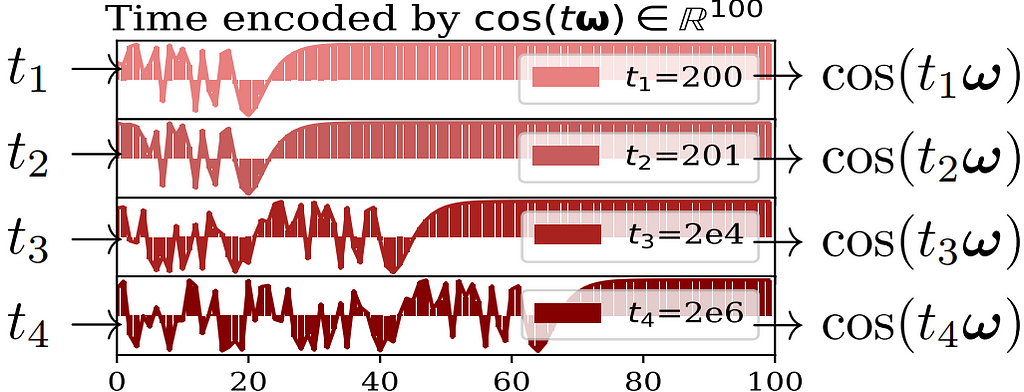
x-axis is the vector dimension and y-axis is the cosine value.
Image source: Cong et al. 2023
Lastly, Suresh et al. pointed out that existing methods maximizes accuracy independently over future links, ignoring the fact that future links often have dependency between each other. This is seen when a user selects among a list of items to purchase or a set of users to connect in a social network. Therefore, Suresh et al. treat dynamic link prediction as a ranking problem and propose Temporal Graph network for RANKing (TGRank) to learn to rank over a list of candidates. The pipeline of TGRank is shown below. The task query now contains a center node s (in the example) with a set of candidate nodes (all other nodes in the subgraph) and the goal is to rank the most likely candidate as the destination of node s. To this end, TGRank follows three steps. First, the node s is labeled differently from other nodes. Then, GNNs are used to diffuse the center node label to every ranking candidate. This parametrized label diffusion step aggregates timestamps, multiplicity as well as features of historical interactions along the network from the center node to all candidates and provides provably more expressive power for link prediction. Lastly, a list-wise loss is used to optimize the ranking amongst candidates jointly. Empirically, it is also shown that with a listwise ranking loss, popular models such as TGN and TGAT also perform better than their original setup with binary classification loss.
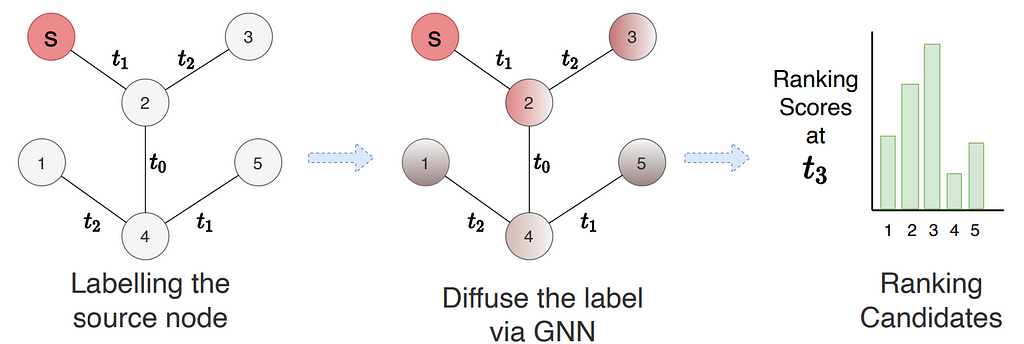
Image source: Suresh et al. 2023
Spatiotemporal Graphs and Graph Deep Learning for Time Series Processing
“Basing our predictions primarily on the most related observations is sensible, yet not always straightforward, as relevant data relations often hide in plain sight. Unveiling them is a captivating challenge, particularly when they are dynamic or involve more than two entities.” — Daniele Zambon, PostDoc at The Swiss AI Lab IDSIA
In the temporal graph learning community, the term spatiotemporal graph has been often used to indicate a graph with fixed topology and node features that change over time, usually at discrete time steps corresponding to regularly sampled observations. More recently the problem of processing data with such a structure is being considered from a different perspective, i.e., by considering the dynamic node feature as time series and edges as functional dependencies among sequences of observations (Cini et al. 2023, Ming et al. 2023). From this perspective, which significantly deviates from many of the settings discussed elsewhere in this blog post, spatiotemporal graph-based representations allow for processing collections of correlated time series by taking advantage of the architectural biases typical of graph neural networks.
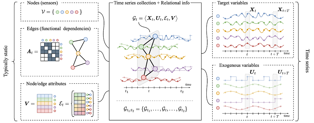
Image source: Cini et al. 2023, by authors.
Such sets of correlated time series can be generated by sensors, either physical or not. An example is in the traffic domain, where time series might correspond to readings of sensors measuring the number of vehicles passing by at a crossroads. Each sensor will correspond to a different node and an adjacency matrix can be obtained, for instance, by joining with an edge only those sensors directly connected by a road segment. Besides traffic forecasting (Li et al. 2018, Yu et al. 2018), these representations have been used in a wide range of time series processing applications ranging from air quality monitoring (Chen et al. 2021) and energy analytics (Cini et al. 2023) to biomedical data processing (Zhang et al. 2022) and financial time series analysis (Matsunaga et al. 2019).

Image source: tutorial at ECML PKDD 2023 by authors.
To process this data, the standard message-passing framework needs to be updated to handle sequences of observations coming from the neighborhood of each node. This can easily be done by replacing the proper operators (i.e., the message and update functions) with operators able to process the data along the temporal dimension, e.g., recurrent cells (Seo et al. 2018), spatiotemporal convolutions (Wu et al. 2019) and attention-based architectures (Marisca et al. 2022). The resulting models are known as spatiotemporal graph neural networks (STGNNs) and there has been a large amount of research dedicated to coming up with effective architectures (see Ming et al. 2023). One of the main advantages of using STGNNs is that the same set of parameters can be used to forecast any subset of time series, while taking dependencies into account throughout the processing. This is a massive advantage over standard multivariate time series forecasting models that usually would have to forecast each time series separately or give up parameter sharing. Hybrid STGNNs, with some time-series-specific parameters, can also be considered and, as we have shown in a recent NeurIPS paper, often outperform models where all parameters are shared. Besides the model architecture, graph-based representations, as shown by Zambon et al., can also help in assessing the optimality of a forecasting model by focusing the spatiotemporal correlation analysis to interconnected nodes.
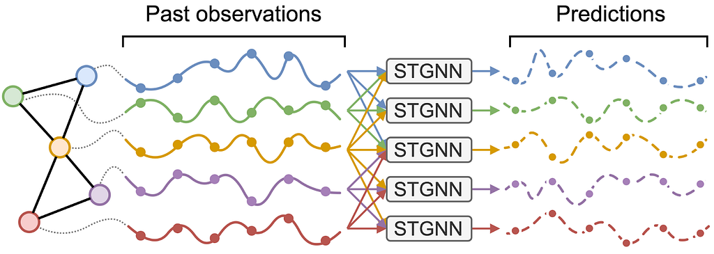
Image by authors.
Several challenges are inherent to the field, starting from dealing with irregularly sampled time series and missing data; indeed, both are quite common phenomena when dealing with actual cyber-physical systems. Luckily, graph-based models are useful in this context as well, for example allowing to condition the reconstruction on observations at neighboring sensors. Scalability is another major concern as differently from standard GNNs, message-passing is often performed w.r.t. each time step. Existing scalable architectures mostly rely on subsampling and/or pre-computed node features. When no prior relation information is available, the challenge becomes that of learning a latent graph directly from the time series. The problem has been tackled, for example, by directly learning an adjacency matric (e.g., Wu et al. 2019) or, under a probabilistic framework, by relying on reparametrization tricks and score-based estimators.

Image source: Cini et al. 2023. by authors
Since this topic was not covered in last year’s blog post, the objective here was to give a short overview of the settings and the problems that can be modeled. Many directions are currently being explored, from graph state-space models and graph Kalman filters to diffusion-based and continuous space-time models. If you are interested in knowing more and/or using these models in practice, we recently released a comprehensive tutorial paper on the topic. You can also check out Torch Spatiotemporal (tsl), our library to build graph-based time series processing pipelines.
- Tutorial paper: Graph Deep Learning for Time Series Forecasting
- Library: Torch Spatiotemporal (tsl)
Temporal Knowledge Graph
There were surprisingly few temporal KG papers in this year’s top ML conferences: TILP (Xiong et al. 2023) on deriving temporal rule learning competitive with neural methods, and theory work by Chen and Wang to measure expressiveness of temporal GNNs. In fact, the most interesting (to me) papers on this topic were found at the TGL workshop at NeurIPS’23 (one more reason for you to follow the venue!), e.g., predicting future time intervals by Pop and Kostylev, or identifying leakages in standard benchmarking datasets by Pan et al. Finally, I’d outline the Unified Urban KG (UUKG) by Ning et al as a fresh look on temporal KG datasets that actually make practical sense and a use-case — modeling transportation flows in the city.
UUKG illustrates the biggest problem of the shrinking temporal KG community — the lack of practically important tasks and datasets where it would be possible to demonstrate the utility of the data modeling paradigm in real-world tasks. That is, adding 1% of MRR/Hits@10 on 10-year old KG embedding benchmarks is rather useless these days compared to the successes of Geometric Deep Learning in biology or materials science (or compared to LLMs, but that’s a story for another day). Hopefully, we will see more UUKG-like practically useful datasets.
Perhaps another adjacent area where temporal KGs might make a difference is heterogeneous graphs (that usually have typed edges) that are much more used in industry. For example, the recent RelBench (Relational Deep Learning Benchmark) formulates a temporal prediction problem over relational databases that can be easily converted to KGs or hypergraphs.
Causality-Aware Temporal Graph Learning
“Einstein said the arrow of time flies in only one direction. […] And who among us, offered the chance, would not relive the day or hour in which we first knew love, or ecstasy, or made a choice that forever altered our future, negating a life we might have had? Such chances are rarely granted.” — Greg Iles, The Quiet Game
One reason why temporal graph learning is interesting is that — depending on the data at hand — it requires different perspectives. As an example, consider temporal graphs data with high-resolution (possibly continuous) time stamps. In such data, discrete-time graph learning techniques that utilize sequences of snapshot graphs require a coarse-graining of time, where each snapshot consists of edges occurring in a certain time interval. This coarse-graining allows to generalize (static) graph learning techniques to time series data. But it introduces a major issue: Each snapshots discards information on the temporal order in which edges occurred, which is the foundation of causal or time-respecting paths (Kempe et al. 2000). Like paths in static graphs, time-respecting paths are important since they tell us which nodes can causally influence each other indirectly. Below, we illustrate this in a simple temporal graph with two undirected edges (a,b) and (b,c) occurring at times t₁ and t₂ respectively. If (a,b) occurs before (b,c), a can causally influence c via a time-respecting path (indicated in purple) passing through b. If the temporal order of edges is reversed, a cannot causally influence c, since any influence must propagate backwards in time. Note that the directedness of the influence from a to c is due to the directed arrow of time and despite the fact that both edges are undirected. Moreover, while two edges (a,b) and (b,c) in a static, time-aggregated graph imply a transitive path from a via b to c (purple) and vice-versa (orange), this is not true for temporal graphs.
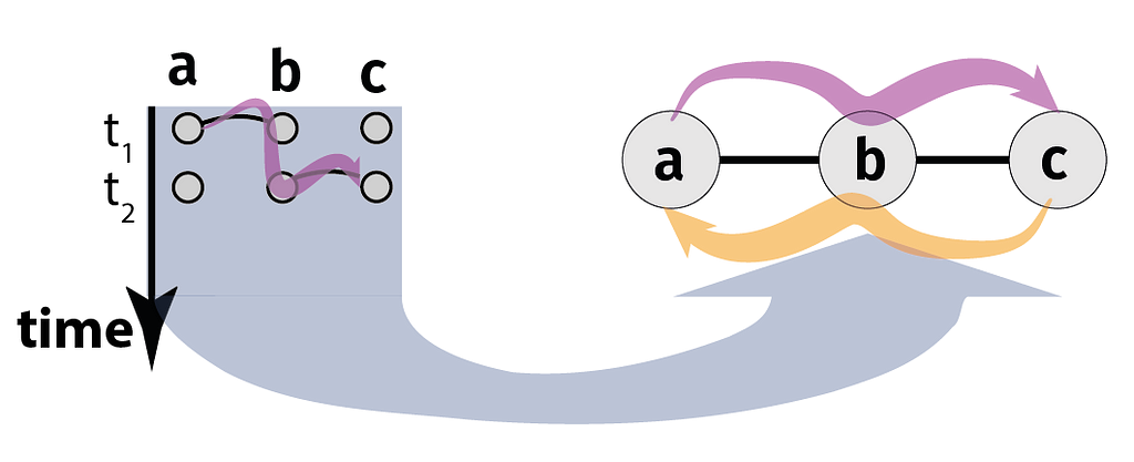
Image by authors.
Several works have shown that — due to the arrow of time — the causal topology of temporal graphs, i.e. which nodes can possibly causally influence each other via time-respecting paths, strongly differs from their static counterparts, with interesting implications for epidemic spreading (Pfitzner et al. 2013), diffusion speed (Scholtes et al. 2014), node centralities (Rosvall et al. 2014), or community detection (Lambiotte et al. 2019). Can we make deep learning methods aware of patterns in the causal topology of temporal graphs? Advances presented at this year show that this can be achieved based on models that generalize commonly used static representations of temporal graphs. Consider a weighted time-aggregated graph, where a (directed) edge (a,b) with weight five captures that (a,b) occurred five times in a temporal graph. Such a weighted, time-aggregated graph is illustrated in the bottom of panel 2 in the figure below.
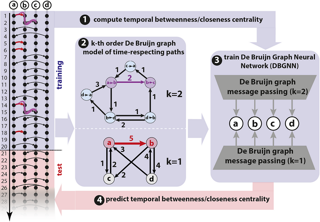
Image source: Heeg et al., by authors
Each edge in the temporal graph is a time-respecting path with length one. A weighted time-aggregated graph thus corresponds to a first-order model for the causal topology of a temporal graph, which captures time-respecting paths of length one. It neglects the temporal ordering of edges, since we only count how often each edge occurred. A line graph transformation enables us to generalize this idea to causality-aware models that facilitate temporal graph learning: We simply replace edges in the first-order graph by nodes in a second-order graph, i.e. we turn edges (a,b) and (b,c) into nodes “a→b” and “b→c”, respectively. In the resulting second-order graph (see the top graph in panel 2 in figure), we can use edges to represent time-respecting paths of length two, i.e. edge (a→b, b→c) indicates that a causally influence c via b. However, the reverse order of edges are not included. If the edges occur in reverse order, we do not include (a→b, b→c). Importantly, such a second-order graph is sensitive to the temporal ordering of edges, while a first-order graph is not! In Scholtes, 2017, this is generalized to higher orders, which yields k-th order De Bruijn graph models for the causal topology of temporal graphs.
Qarkaxhija et al. have shown that neural message passing in such higher-order De Bruijn graphs yields a causality-aware graph neural network architecture for temporal graphs. Building on these De Bruijn Graph Neural Networks (DBGNN), in a poster at this year’s TGL workshop, Heeg and Scholtes address the challenge to predict temporal betweenness and closeness centralities of nodes. Since they are influenced by the arrow of time, temporal node centralities can drastically differ from static centralities. Moreover, it is costly to compute them! This is addressed by training a DBGNN model on a first time interval of a temporal graph, then using the trained model to forecast temporal centralities in the remaining data. The overall approach is illustrated above. Empirically results are promising and showcased the potential of causality-aware graph learning. We also hope to see more attention from the community in learning causal structure on temporal graphs in 2024.
Interested in causality-aware temporal graph learning? Then there’s good news! The techniques above are implemented in the Open Source library pathpyG, which builds on PyG. There is an introductory video and a tutorial available. A recorded talk given in the temporal graph reading group provides an in-depth introduction of the underlying research.
Explainable Temporal Graph Methods
“Most important graph-structured data in real-world settings are temporal in nature. Explainable temporal graph models have the potential to unveil the long-standing questions on effective strategies and knowledge that can be leveraged to make temporal predictions, enabling extraction of insights from deep learning models and assisting scientific discovery and forecasting.” — Rex Ying, Assistant Professor, Yale University
2023 saw the first approaches for explaining temporal GNN methods. Explainers are important for high-stake applications such as fraud detection and disease progression prediction in healthcare. Xia et al. proposed T-GNNExplainer as the first explainer designed for temporal graph models. T-GNNExplainer is model-agnostic and finds important events from a set of candidate events to best explain the model prediction. Xia et al. treat the problem of identifying a subset of explaining events as a combinatorial optimization problem by searching over a subset of the temporal graph within a given size. To tackle this, T-GNNExplainer employs an explorer-navigator framework. The navigator is trained from multiple target events to capture inductive correlations between events while the explorer searches out a specific combination of events based on Monte Carlo Tree Search, including node selection, node expansion, reward simulation and backprop. Which events are pruned is inferred from the navigator. The diagram below shows the framework of T-GNNExplainer.

Image source: Xia et al. 2023
Recently, Chen et al. argued that to form human intelligible explanations for temporal graph events requires the explanation to be events that are temporally proximate and spatially adjacent to that of the prediction, referred to as cohesive explanations. Utilizing temporal motifs, recurring substructures within the temporal graph, is a natural solution to form cohesive explanations for temporal graphs. This is because temporal motifs are crucial factors that guide the generative process of future events. In the following example, the preferential attachment rule (often facilitating influencer effect in e-commerce) and triadic closure rule (explains common-friend rules in social networks) forms cohesive and plausible explanations.

Image source: Chen et al. 2023
Therefore, Chen et al. proposed TempME, a novel Temporal Motif-based Explainer to identify important temporal motifs to explain temporal GNNs. The framework of TempME is shown in the below figure. First, temporal motifs surrounding the target prediction are extracted. Then these candidate motifs are encoded via the Motif Encoder which leverages event anonymization, message passing and graph pooling to generate an embedding for each motif. Then, based on the Information-bottleneck principle, TempME assigns importance scores to these motifs constrained by both explanation accuracy and information compression. Lastly, explanations are constructed by sampling from the Bernoulli distribution based on the importance score.

Image credit: Chen et al. 2023
Adversarial Attacks on Temporal Graphs
“As temporal graphs are adopted to be used for important tasks, like fraud detection, it is important to understand their failure points under adversarial attacks. Understanding and quantifying such blind spots is the first step towards creating robust and reliable temporal GNN models. Such efforts are necessary to ensure industry adoption of these models.” – Srijan Kumar, Assistant Professor at Georgia Institute of Technology
Adversarial attacks can target the privacy of customers or affect critical decisions in financial systems. As temporal graph models are deployed to applications such as recommendation systems and fraud detection, it is important to investigate attacks and design defense mechanisms for TG models. Chen et al. proposed the first adversarial attack for dynamic link prediction called Time-aware Gradient Attack (TGA) for discrete time dynamic graphs. TGA rewires a limited number of links from the original network and the most valuable links to the predicted link are determined by the gradient information generated by the TG model.

The attacker can flip the prediction of the model while evading detection.
Image source: Sharma et al. 2023
Recently, Sharma et al. argued that effective attacks on temporal graphs must optimize both edge and time perturbations while preserving the original graph evolution. This is because drastic attacks that disturb the graph evolution would be easily detected by anomaly detection methods. Therefore, Sharma et al. formulated evolution-preserving attacks on discrete-time dynamic graphs as the Temporal Dynamics-Aware Perturbation (TDAP) constraint. TDAP asserts that perturbations added at a given timestamp must only be a small fraction of the actual number of changes with respect to the preceding timestamp. TDAP is shown to preserve the rate of change in both the structure and the embedding spaces. An overview of TDAP is shown in the figure below. Sharma et al. then proposes a novel attack method called Temporal Dynamics-aware Projected Gradient Descent (TD-PGD) which is shown to have a closed-form projection operator under the TDAP constraint. An online version of TD-PGD is also proposed where perturbations can be added in real time. Lastly, it is shown empirically that TDAP-constrained perturbations can indeed evade attacks by embedding-based anomaly detection methods.
Libraries and Benchmarks
In 2023 saw a significant push towards standardized libraries and benchmarks for temporal graph learning. TGB provides an open and standardized benchmark for node and link level tasks. DyGLib is a library which includes standard training pipelines, extensible coding interfaces, and comprehensive evaluation strategies for temporal graph learning. Zhang et al. introduced the novel concept of Live Graph Lab, providing live graphs according to blockchain transactions. With a set of tools for downloading, parsing, cleaning, and analyzing blockchain transactions, Live Graph Lab offers researchers the opportunity to extract update to date temporal graph data any time and use it for analysis or testing. Zhou et al. noticed that node memory used in TG models favors small batch sizes and needs to be maintained synchronously across all trainers. Therefore, they proposed DistTGL, an efficient and scalable solution to train memory-based TGNNs on distributed GPU clusters. Enabling multi-GPU training on large datasets is an important direction to deploy TG models on large datasets. We present an updated list of libraries and benchmarks for temporal graph learning:
- TGB website and pypi install
- DyGLib Github
- Live Graph Lab website and dataset
- DistTGL Github
- Torch Spatiotemporal (TSL) website and Github
- pathpyG website and Github
- RelBench website and Github
- Pytorch Geometric Temporal
- TGL paper and Github
- DGB pypi install, paper and datasets
- Chartalist Blockchain Network website, paper and Github
- TKG Forecasting Evaluation paper and Github
Joining Temporal Graph Learning Community
To join the fast growing TG community, sign up for the weekly temporal graph reading group here. Visit the reading group website and Youtube to see all upcoming and recorded past talks. We also include the invitation link to the TG slack on the website (updated monthly). The second edition of temporal graph learning workshop @ NeurIPS 2023 includes an exciting lineup of 35 posters for cutting edge research in TG. You can also find the talk recordings on the NeurIPS virtual site (will be public in a month). If you want to be a reviewer for the next edition of the workshop, sign up here. To find more about the research from the authors of this post, see our websites: Shenyang(Andy) Huang, Emanuele Rossi, Michael Galkin ,Andrea Cini and Ingo Scholtes. Hope to see you at the reading group or the next edition of the workshop!
Image by authors.
Temporal Graph Learning in 2024 was originally published in Towards Data Science on Medium, where people are continuing the conversation by highlighting and responding to this story.
Originally appeared here:
Temporal Graph Learning in 2024

