Tag: technews

  • What to expect at Samsung’s Galaxy S25 Unpacked event

    Will Shanklin

    Samsung’s big Galaxy S25 launch is right around the corner. The first Galaxy Unpacked event of 2025 is confirmed for January 22 at 1PM ET in San Jose, CA, where Samsung’s “Next Big Thing” (to borrow a 14-year-old marketing slogan) will be revealed. What exactly will be on tap? Well, apart from a few sure bets and some likely leaks, only those sworn to a blood oath under an NDA know for certain. But here are the most likely products and features we’ll see.

    Photo of the Samsung Galaxy S24 Ultra phone sitting in the snow.
    Galaxy S24 Ultra
    Sam Rutherford for Engadget

    Much like Apple reveals its latest iPhones at its first fall event, Samsung typically launches its mainline Galaxy S flagships at its first Unpacked shindig of the year. You can bet the farm that there will be Galaxy S25 phones at this event. And given Samsung’s recent trend of launching three tiers of flagships — standard, Plus and Ultra — you can bet we’ll see that again. (Samsung could technically change the brand names, but the three-layered lineup is practically guaranteed.) There’s even an FCC certification (first spotted by 91Mobiles) to dispel any doubts.

    The degree of certainty falls sharply once we dig into the phones’ features. A subtle redesign with rounded corners, flatter edges and thinner bezels appears likely based on a leaked video posted to Reddit and images from reputable tipster Ice Universe. But this isn’t expected to be the generation where Samsung’s hiring of a former Mercedes-Benz designer will lead to drastic aesthetic changes.

    Promo image breaking down the Qualcomm Snapdragon 8 Elite’s features.
    Qualcomm

    At least in the US, the phone is practically guaranteed to use Qualcomm’s Snapdragon 8 Elite processor, which the chip-maker revealed in October. (Qualcomm even listed Samsung among the companies launching devices with that processor “in the coming weeks.”) Like just about every flagship processor these days, the Snapdragon 8 Elite is built for on-device generative AI, which aligns with Samsung’s Galaxy AI blitz in recent models.

    We don’t know whether the company will split its S25 processors between Snapdragon (US and other markets) and Exynos (everywhere else), but Ice Universe has claimed it will be all Snapdragon this generation. That would be a good thing, given what’s often a glaring performance and battery life disparity favoring Qualcomm.

    The phone will run Samsung’s One UI 7 on top of Android 15. We know this because Samsung said in October that its user experience (based on Android 15) will launch on the next Galaxy S flagships. It’s already available in beta for Galaxy S24 phones.

    Samsung Executive Vice President Sally Hyesoon Jeong onstage in front of the text
    Samsung

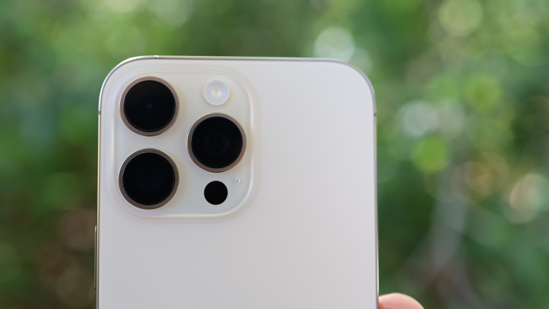
    Samsung is rumored to stick with last-generation OLED displays (made with M13 organic materials) instead of the brighter and more efficient M14 OLED panels used in the iPhone 16 Pro and Google Pixel 9. Logic suggests Samsung would want its best homemade screen in its best phones — especially when its competitors are already using it. But it could stick with the cheaper panels to keep the bill of materials down. Perhaps it calculated that better displays don’t make for better generative AI (the obsession of nearly every tech company right now), while the latest Qualcomm chip does.

    Speaking of AI, expect Samsung to devote a perhaps agonizingly long portion of the event to generative AI features. The hit-or-miss DigiTimes reported last month that the Galaxy S25 series will include “an AI Agent that provides personalized clothing suggestions and transport information.” What that would look like in practice is anyone’s guess, but I’m not sure I want to know.

    Photo of the back of the Samsung Galaxy S24 Ultra. Closeup of the camera lenses.
    Galaxy S24 Ultra
    Sam Rutherford for Engadget

    On the camera front, Ice Universe claims (via Android Headlines) it’s “confirmed” that only the ultra-wide sensor will see an upgrade in the Galaxy S25 Ultra — to 50MP from 12MP in last year’s model. The leaker says the S25 Ultra will stick with a 200MP main sensor, 10MP 3x zoom and 50MP 5x zoom.

    Samsung will add the Qi2 wireless charging standard to its new flagships — and that comes straight from the horse’s (aka, the Wireless Power Consortium’s) mouth. However, leaker chunvn8888 (aka “yawn”) says Samsung’s phones won’t have built-in magnets for Qi2’s native MagSafe in everything but name charging. Instead, the leaker says Samsung will sell a first-party case with a Qi2 magnetic ring to enable that. (Gotta move those accessories, baby!)

    Rumors have buzzed about an alleged Galaxy S25 Slim with a — you guessed it — slimmer design joining the trio at some point this year. That’s something Apple is also rumored to be working on. However, given the FCC certifications only appear to cover the familiar trio of flagships, that phone (if it’s in the pipeline at all) may not arrive until later in the year.

    A hand wearing the Samsung Galaxy Ring.
    Galaxy Ring
    Sam Rutherford for Engadget

    DigiTimes reported in December that Samsung would show off (or maybe just tease) the Galaxy Ring 2 and augmented reality (AR) glasses during its January Unpacked event.

    The Taiwanese publication says the Galaxy Ring 2 will add two more sizes to the nine from the original model, which only launched in July. The second-gen wearable health tracker is said to add new AI features (surprise!) and updated sensors for more accurate measurements. The Galaxy Ring 2 is also rumored to last longer than the current model’s maximum of seven days.

    A tech bro wearing a prototype of Android XR glasses in a modern posh office.
    Google

    DigiTimes also claims Samsung’s AR glasses — which the company has confirmed it’s working on — will look like regular prescription glasses and weigh around 50g. It says the futuristic glasses would use Google’s Gemini AI, which aligns with what we already know about Samsung’s partnership with Google and Qualcomm on Android XR. But given the lack of supply chain rumors surrounding the glasses, it’s likely that any mention at the event would amount to little more than a teaser, a la its grand reveal of… a stinkin’ render for the first Galaxy Ring at Unpacked 2024.

    We also know Samsung is co-developing an Android XR (extended reality) headset — codenamed Project Moohan — alongside Google and Qualcomm. The “lightweight” and “ergonomically designed” headset will have a “state-of-the-art display,” passthrough video and natural multi-modal input. Google’s renderings show a wearable reminiscent of Apple’s $3,500 Vision Pro.

    Render of an Android XR headset.
    Project Moohan
    Google / Samsung

    Since Google only recently began offering a developer kit and API for the platform, any glimpse of it at Unpacked wouldn’t likely include an imminent release or deep dive into its hardware.

    Engadget will have full coverage of Samsung’s first Unpacked event of 2025. More to come on January 22!

    This article originally appeared on Engadget at https://www.engadget.com/mobile/smartphones/what-to-expect-at-samsungs-galaxy-s25-unpacked-event-182028420.html?src=rss

    Go Here to Read this Fast! What to expect at Samsung’s Galaxy S25 Unpacked event

    Originally appeared here:
    What to expect at Samsung’s Galaxy S25 Unpacked event

  • Exploring New Hyperparameter Dimensions with Laplace Approximated Bayesian Optimization

    Exploring New Hyperparameter Dimensions with Laplace Approximated Bayesian Optimization

    Arnaud Capitaine

    Is it better than grid search?

    Image by author from canva

    When I notice my model is overfitting, I often think, “It is time to regularize”. But how do I decide which regularization method to use (L1, L2) and what parameters to choose? Typically, I perform hyperparameter optimization by means of a grid search to select the settings. However, what happens if the independent variables have different scales or varying levels of influence? Can I design a hyperparameter grid with different regularization coefficients for each variable? Is this type of optimization feasible in high-dimensional spaces? And are there alternative ways to design regularization? Let’s explore this with a hypothetical example.

    Use case

    My fictional example is a binary classification use case with 3 explanatory variables. Each of these variables is categorical and has 7 different categories. My reproducible use case is in this notebook. The function that generates the dataset is the following:

    import numpy as np
    import pandas as pd

    def get_classification_dataset():
    n_samples = 200
    cats = ["a", "b", "c", "d", "e", "f"]
    X = pd.DataFrame(
    data={
    "col1": np.random.choice(cats, size=n_samples),
    "col2": np.random.choice(cats, size=n_samples),
    "col3": np.random.choice(cats, size=n_samples),
    }
    )
    X_preprocessed = pd.get_dummies(X)

    theta = np.random.multivariate_normal(
    np.zeros(len(cats) * X.shape[1]),
    np.diag(np.array([1e-1] * len(cats) + [1] * len(cats) + [1e1] * len(cats))),
    )

    y = pd.Series(
    data=np.random.binomial(1, expit(np.dot(X_preprocessed.to_numpy(), theta))),
    index=X_preprocessed.index,
    )
    return X_preprocessed, y

    For information, I deliberately chose 3 different values for the theta covariance matrix to showcase the benefit of the Laplace approximated bayesian optimization method. If the values were somehow similar, the interest would be minor.

    Benchmark

    Along with a simple baseline model that predicts the mean observed value on the training dataset (used for comparison purposes), I opted to design a slightly more complex model. I decided to one-hot encode the three independent variables and apply a logistic regression model on top of this basic preprocessing. For regularization, I chose an L2 design and aimed to find the optimal regularization coefficient using two techniques: grid search and Laplace approximated bayesian optimization, as you may have anticipated by now. Finally, I evaluated the model on a test dataset using two metrics (arbitrarily selected): log loss and AUC ROC.

    Before presenting the results, let’s first take a closer look at the bayesian model and how we optimize it.

    Bayesian model

    In the bayesian framework, the parameters are no longer fixed constants, but random variables. Instead of maximizing the likelihood to estimate these unknown parameters, we now optimize the posterior distribution of the random parameters, given the observed data. This requires us to choose, often somewhat arbitrarily, the design and parameters of the prior. However, it is also possible to treat the parameters of the prior as random variables themselves — like in Inception, where the layers of uncertainty keep stacking on top of each other…

    In this study, I have chosen the following model:

    I have logically chosen a bernouilli model for Y_i | θ, a normal centered prior corresponding to a L2 regularization for θ | Σ and finally for Σ_i^{-1}, I chose a Gamma model. I chose to model the precision matrix instead of the covariance matrix as it is traditional in the literature, like in scikit learn user guide for the Bayesian linear regression [2].

    In addition to this written model, I assumed the Y_i and Y_j are conditionally (on θ) independent as well as Y_i and Σ.

    Calibration

    Likelihood

    According to the model, the likelihood can consequently be written:

    In order to optimize, we need to evaluate nearly all of the terms, with the exception of P(Y=y). The terms in the numerators can be evaluated using the chosen model. However, the remaining term in the denominator cannot. This is where the Laplace approximation comes into play.

    Laplace approximation

    In order to evaluate the first term of the denominator, we can leverage the Laplace approximation. We approximate the distribution of θ | Y, Σ by:

    with θ* being the mode of the mode the density distribution of θ | Y, Σ.

    Even though we do not know the density function, we can evaluate the Hessian part thanks to the following decomposition:

    We only need to know the first two terms of the numerator to evaluate the Hessian which we do.

    For those interested in further explanation, I advise part 4.4, “The Laplace Approximation”, from Pattern Recognition and Machine Learning from Christopher M. Bishop [1]. It helped me a lot to understand the approximation.

    Laplace approximated likelihood

    Finally the Laplace approximated likelihood to optimize is:

    Once we approximate the density function of θ | Y, Σ, we could finally evaluate the likelihood at whatever θ we want if the approximation was accurate everywhere. For the sake of simplicity and because the approximation is accurate only close to the mode, we evaluate approximated likelihood at θ*.

    Here after is a function that evaluates this loss for a given (scalar) σ²=1/p (in addition to the given observed, X and y, and design values, α and β).

    import numpy as np
    from scipy.stats import gamma

    from module.bayesian_model import BayesianLogisticRegression

    def loss(p, X, y, alpha, beta):
    # computation of the loss for given values:
    # - 1/sigma² (named p for precision here)
    # - X: matrix of features
    # - y: vector of observations
    # - alpha: prior Gamma distribution alpha parameter over 1/sigma²
    # - beta: prior Gamma distribution beta parameter over 1/sigma²

    n_feat = X.shape[1]
    m_vec = np.array([0] * n_feat)
    p_vec = np.array(p * n_feat)

    # computation of theta*
    res = minimize(
    BayesianLogisticRegression()._loss,
    np.array([0] * n_feat),
    args=(X, y, m_vec, p_vec),
    method="BFGS",
    jac=BayesianLogisticRegression()._jac,
    )
    theta_star = res.x

    # computation the Hessian for the Laplace approximation
    H = BayesianLogisticRegression()._hess(theta_star, X, y, m_vec, p_vec)

    # loss
    loss = 0
    ## first two terms: the log loss and the regularization term
    loss += baysian_model._loss(theta_star, X, y, m_vec, p_vec)
    ## third term: prior distribution over sigma, written p here
    out -= gamma.logpdf(p, a = alpha, scale = 1 / beta)
    ## fourth term: Laplace approximated last term
    out += 0.5 * np.linalg.slogdet(H)[1] - 0.5 * n_feat * np.log(2 * np.pi)

    return out

    In my use case, I have chosen to optimize it by means of Adam optimizer, which code has been taken from this repo.

    def adam(
    fun,
    x0,
    jac,
    args=(),
    learning_rate=0.001,
    beta1=0.9,
    beta2=0.999,
    eps=1e-8,
    startiter=0,
    maxiter=1000,
    callback=None,
    **kwargs
    ):
    """``scipy.optimize.minimize`` compatible implementation of ADAM -
    [http://arxiv.org/pdf/1412.6980.pdf].
    Adapted from ``autograd/misc/optimizers.py``.
    """
    x = x0
    m = np.zeros_like(x)
    v = np.zeros_like(x)

    for i in range(startiter, startiter + maxiter):
    g = jac(x, *args)

    if callback and callback(x):
    break

    m = (1 - beta1) * g + beta1 * m # first moment estimate.
    v = (1 - beta2) * (g**2) + beta2 * v # second moment estimate.
    mhat = m / (1 - beta1**(i + 1)) # bias correction.
    vhat = v / (1 - beta2**(i + 1))
    x = x - learning_rate * mhat / (np.sqrt(vhat) + eps)

    i += 1
    return OptimizeResult(x=x, fun=fun(x, *args), jac=g, nit=i, nfev=i, success=True)

    For this optimization we need the derivative of the previous loss. We cannot have an analytical form so I decided to use a numerical approximation of the derivative.

    Inference

    Once the model is trained on the training dataset, it is necessary to make predictions on the evaluation dataset to assess its performance and compare different models. However, it is not possible to directly calculate the actual distribution of a new point, as the computation is intractable.

    It is possible to approximate the results with:

    considering:

    Results

    I chose an uninformative prior over the precision random variable. The naive model performs poorly, with a log loss of 0.60 and an AUC ROC of 0.50. The second model performs better, with a log loss of 0.44 and an AUC ROC of 0.83, both when hyperoptimized using grid search and bayesian optimization. This indicates that the logistic regression model, which incorporates the dependent variables, outperforms the naive model. However, there is no advantage to using bayesian optimization over grid search, so I’ll continue with grid search for now. Thanks for reading.

    … But wait, I am thinking. Why are my parameters regularized with the same coefficient? Shouldn’t my prior depend on the underlying dependent variables? Perhaps the parameters for the first dependent variable could take higher values, while those for the second dependent variable, with its smaller influence, should be closer to zero. Let’s explore these new dimensions.

    Benchmark 2

    So far we have considered two techniques, the grid search and the bayesian optimization. We can use these same techniques in higher dimensions.

    Considering new dimensions could dramatically increase the number of nodes of my grid. This is why the bayesian optimization makes sense in higher dimensions to get the best regularization coefficients. In the considered use case, I have supposed there are 3 regularization parameters, one for each independent variable. After encoding a single variable, I assumed the generated new variables all shared the same regularization parameter. Hence the total regularization parameters of 3, even if there are more than 3 columns as inputs of the logistic regression.

    I updated the previous loss function with the following code:

    import numpy as np
    from scipy.stats import gamma

    from module.bayesian_model import BayesianLogisticRegression

    def loss(p, X, y, alpha, beta, X_columns, col_to_p_id):
    # computation of the loss for given values:
    # - 1/sigma² vector (named p for precision here)
    # - X: matrix of features
    # - y: vector of observations
    # - alpha: prior Gamma distribution alpha parameter over 1/sigma²
    # - beta: prior Gamma distribution beta parameter over 1/sigma²
    # - X_columns: list of names of X columns
    # - col_to_p_id: dictionnary mapping a column name to a p index
    # because many column names can share the same p value

    n_feat = X.shape[1]
    m_vec = np.array([0] * n_feat)
    p_list = []
    for col in X_columns:
    p_list.append(p[col_to_p_id[col]])
    p_vec = np.array(p_list)

    # computation of theta*
    res = minimize(
    BayesianLogisticRegression()._loss,
    np.array([0] * n_feat),
    args=(X, y, m_vec, p_vec),
    method="BFGS",
    jac=BayesianLogisticRegression()._jac,
    )
    theta_star = res.x

    # computation the Hessian for the Laplace approximation
    H = BayesianLogisticRegression()._hess(theta_star, X, y, m_vec, p_vec)

    # loss
    loss = 0
    ## first two terms: the log loss and the regularization term
    loss += baysian_model._loss(theta_star, X, y, m_vec, p_vec)
    ## third term: prior distribution over 1/sigma² written p here
    ## there is now a sum as p is now a vector
    out -= np.sum(gamma.logpdf(p, a = alpha, scale = 1 / beta))
    ## fourth term: Laplace approximated last term
    out += 0.5 * np.linalg.slogdet(H)[1] - 0.5 * n_feat * np.log(2 * np.pi)

    return out

    With this approach, the metrics evaluated on the test dataset are the following: 0.39 and 0.88, which are better than the initial model optimized by means of a grid search and a bayesian approach with only a single prior for all the independent variables.

    Metrics achieved with the different methods on my use case.

    The use case can be reproduced with this notebook.

    Limits

    I have created an example to illustrate the usefulness of the technique. However, I have not been able to find a suitable real-world dataset to fully demonstrate its potential. While I was working with an actual dataset, I could not derive any significant benefits from applying this technique. If you come across one, please let me know — I would be excited to see a real-world application of this regularization method.

    Conclusion

    In conclusion, using bayesian optimization (with Laplace approximation if needed) to determine the best regularization parameters may be a good alternative to traditional hyperparameter tuning methods. By leveraging probabilistic models, bayesian optimization not only reduces the computational cost but also enhances the likelihood of finding optimal regularization values, especially in high dimension.

    References

    1. Christopher M. Bishop. (2006). Pattern Recognition and Machine Learning. Springer.
    2. Bayesian Ridge Regression scikit-learn user guide: https://scikit-learn.org/1.5/modules/linear_model.html#bayesian-ridge-regression


    Exploring New Hyperparameter Dimensions with Laplace Approximated Bayesian Optimization was originally published in Towards Data Science on Medium, where people are continuing the conversation by highlighting and responding to this story.

    Originally appeared here:
    Exploring New Hyperparameter Dimensions with Laplace Approximated Bayesian Optimization

    Go Here to Read this Fast! Exploring New Hyperparameter Dimensions with Laplace Approximated Bayesian Optimization