Tag: technews

How to Use LLMs and Controlled Vocabularies for Enhanced Similarity Models

The accompanying code for this tutorial is here.

Recommender systems are how we find much of the content and products we consume, probably including this article. A recommender system is:

“a subclass of information filtering system that provides suggestions for items that are most pertinent to a particular user.” — Wikipedia

Some examples of recommender systems we interact with regularly are on Netflix, Spotify, Amazon, and social media. All of these recommender systems are attempting to answer the same question: given a user’s past behavior, what other products or content are they most likely to like? These systems generate a lot of money — a 2013 study from McKinsey found that, “35 percent of what consumers purchase on Amazon and 75 percent of what they watch on Netflix come from product recommendations.” Netflix famously started an open competition in 2006 offering a one million dollar prize to anyone who could significantly improve their recommendation system. For more information on recommender systems see this article.

Generally, there are three kinds of recommender systems: content based, collaborative, and a hybrid of content based and collaborative. Collaborative recommender systems focus on users’ behavior and preferences to predict what they will like based on what other similar users like. Content based filtering systems focus on similarity between the products themselves rather than the users. For more info on these systems see this Nvidia piece.

Calculating similarity between products that are well-defined in a structured dataset is relatively straightforward. We could identify which properties of the products we think are most important, and measure the ‘distance’ between any two products given the difference between those properties. But what if we want to compare items when the only data we have is unstructured text? For example, given a dataset of movie and TV show descriptions, how can we calculate which are most similar?

In this tutorial, I will:

1. Show a basic similarity model (no controlled vocabulary) of unstructured text using natural language processing (NLP) techniques
2. Create a genre list using an LLM
3. Use the genre list to tag films with genres
4. Use the genre tags to build a similarity model
5. Use the genre tags to create a network visualization

The goal, for me, in writing this, was to learn two things: whether a taxonomy (controlled vocabulary) significantly improved the outcomes of a similarity model of unstructured data, and whether an LLM can significantly improve the quality and/or time required to construct that controlled vocabulary.

If you don’t feel like reading the whole thing, here are my main findings:

• The basic NLP model (without a controlled vocabulary) certainly has some problems — it sometimes uses words for identifying similar movies that are not relevant (like the protagonists’ first name or the location).
• Using a controlled vocabulary does significantly improve the outcomes of the similarity model, at least based on some of the examples I have been using to test the models.
• Building a simple, basic genre list using an LLM is easy — building a useful and/or detailed genre taxonomy is hard i.e. it would take more iterations or more descriptive prompts. I ended up building a quick and dirty list of about 200 genres without definitions, which worked good enough for doing simple similarity calculations.
• Even this very basic genre list built using an LLM has issues, however. There are duplicate genres with minor spelling differences, for example.
• Using an LLM to tag the movies and TV shows took a very long time. This might just be a problem in the way I have structured my code though.
• Perhaps not surprisingly, the depth and breadth of the taxonomy matters. Like I said above, building a detailed and descriptive taxonomy of movie genres is difficult and would require a lot more work than I am willing to do for this tutorial. But depending on the use case, that level of detail might not be necessary. I started by building a taxonomy of thousands of genres with synonyms and definitions but that had drawbacks — the tagging became harder and the similarity calculations were often not as good. Because I was only looking at a couple thousand movies, having a genre list of thousands of genres just made every movie unique and similar to almost nothing.
• Visualizing movies and genres as graphs is awesome, as always.

Basic Similarity Model of Unstructured Text Using NLP Techniques

We could use natural language processing (NLP) to extract key words from the text, identify how important these words are, and then find matching words in other descriptions. Here is a tutorial on how to do that in Python. I won’t recreate that entire tutorial here but here is a brief synopsis:

First, we extract key words from a plot description. For example, here is the description for the movie, ‘Indiana Jones and the Raiders of the Lost Ark.’

“When Indiana Jones is hired by the government to locate the legendary Ark of the Covenant, he finds himself up against the entire Nazi regime.”

We then use out-of-the-box libraries from sklearn to extract key words and rank their ‘importance’. To calculate importance, we use term-frequency-inverse document frequency (tf-idf). The idea is to balance the frequency of the term in the individual film’s description with how common the word is across all film descriptions in our dataset. The word ‘finds,’ for example, appears in this description, but it is a common word and appears in many other movie descriptions, so it is less important than ‘covenant’.

This model actually works very well for films that have a uniquely identifiable protagonist. If we run the similarity model on this film, the most similar movies are: ‘Indiana Jones and the Temple of Doom’, ‘Indiana Jones and the Last Crusade’, and ‘Indiana Jones and the Kingdom of the Crystal Skull’. This is because the descriptions for each of these movies contains the words, ‘Indiana’ and ‘Jones’.

But there are problems here. How do we know the words that are extracted and used in the similarity model are relevant? For example, if I run this model to find movies or TV shows similar to ‘Beavis and Butt-head Do America,” the top result is “Army of the Dead.” If you’re not a sophisticated film and TV buff like me, you may not be familiar with the animated series ‘Beavis and Butt-Head,’ featuring ‘unintelligent teenage boys [who] spend time watching television, drinking unhealthy beverages, eating, and embarking on mundane, sordid adventures, which often involve vandalism, abuse, violence, or animal cruelty.’ The description of their movie, ‘Beavis and Butt-head Do America,’ reads, ‘After realizing that their boob tube is gone, Beavis and Butt-head set off on an expedition that takes them from Las Vegas to the nation’s capital.’ ‘Army of the Dead,’ on the other hand, is a Zack Snyder-directed ‘post-apocalyptic zombie heist film’. Why is Army of the Dead considered similar then? Because it takes place in Las Vegas — both movie descriptions contain the words ‘Las Vegas’.

Another example of where this model fails is that if I want to find movies or TV shows similar to ‘Eat Pray Love,’ the top result is, ‘Extremely Wicked, Shockingly Evil and Vile.’ ‘Eat Pray Love’ is a romantic comedy starring Julia Roberts as Liz Gilbert, a recently divorced woman traveling the world in a journey of self-discovery. ‘Extremely Wicked, Shockingly Evil and Vile,’ is a true crime drama about serial killer Ted Bundy. What do these films have in common? Ted Bundy’s love interest is also named Liz.

These are, of course, cherry-picked examples of cases where this model doesn’t work. There are plenty of cases where extracting key words from text can be a useful way of finding similar products. As shown above, text that contains uniquely identifiable names like Power Rangers, Indiana Jones, or James Bond can be used to find other titles with those same names in their descriptions. Likewise, if the description contains information about the genre of the title, like ‘thriller’ or ‘mystery’, then those words can link the film to other films of the same genre. This has limitations too, however. Some films may use the word ‘dramatic’ in their description, but using this methodology, we would not match these films with film descriptions containing the word ‘drama’ — we are not accounting for synonyms. What we really want is to only use relevant words and their synonyms.

How can we ensure that the words extracted are relevant? This is where a taxonomy can help. What is a taxonomy?

Create a genre taxonomy using an LLM

“A taxonomy (or taxonomic classification) is a scheme of classification, especially a hierarchical classification, in which things are organized into groups or types.” — Wikipedia

Perhaps the most famous example of a taxonomy is the one used in biology to categorize all living organisms — remember domain, kingdom, phylum class, order, family, genus, and species? All living creatures can be categorized into this hierarchical taxonomy.

A note on terminology: ontologies are similar to taxonomies but different. As this article explains, taxonomies classify while ontologies specify. “An ontology is the system of classes and relationships that describe the structure of data, the rules, if you will, that prescribe how a new category or entity is created, how attributes are defined, and how constraints are established.” Since we are focused on classifying movies, we are going to build a taxonomy. However, for the purposes of this tutorial, I just need a very basic list of genres, which can’t even really be described as a taxonomy. A list of genres is just a tag set, or a controlled vocabulary.

For this tutorial, we will focus only on genre. What we need is a list of genres that we can use to ‘tag’ each movie. Imagine that instead of having the movie, ‘Eat Pray Love’ tagged with the words ‘Liz’ and ‘true’, it were tagged with ‘romantic comedy’, ‘drama’, and ‘travel/adventure’. We could then use these genres to find other movies similar to Eat Pray Love, even if the protagonist is not named Liz. Below is a diagram of what we are doing. We use a subset of the unstructured movie data, along with GPT 3.5, to create a list of genres. Then we use the genre list and GPT 3.5 to tag the unstructured movie data. Once our data is tagged, we can run a similarity model using the tags as inputs.

I couldn’t find any free movie genre taxonomies online, so I built my own using a large language model (LLM). I started with this tutorial, which used an LLM agent to build a taxonomy of job titles. That LLM agent looks for job titles from job descriptions, creates definitions and responsibilities for each of these job titles, and synonyms. I used that tutorial to create a movie genre taxonomy, but it was overkill — we don’t really need to do all of that for the purposes of this tutorial. We just need a very basic list of genres that we can use to tag movies. Here is the code I used to create that genre list.

I used Netflix movie and TV show description data available here (License CC0: Public Domain).

Import required packages and load english language NLP model.

import openai
import os
import re
import pandas as pd
import spacy
from ipywidgets import FloatProgress
from tqdm import tqdm

# Load English tokenizer, tagger, parser and NER
nlp = spacy.load("en_core_web_sm")

Then we need to set up our connection with OpenAI (or whatever LLM you want to use).

os.environ["OPENAI_API_KEY"] = "XXXXXX"  # replace with yours

Read in the Netflix movie data:

movies = pd.read_csv("netflix_titles.csv")
movies = movies.sample(n=1000) #I just used 1000 rows of data to reduce the runtime

Create a function to predict the genre of a title given its description:

def predict_genres(movie_description):
    prompt = f"Predict the top three genres (only genres, not descriptions) for a movie with the following description: {movie_description}"
    response = openai.completions.create(
      model="gpt-3.5-turbo-instruct",  # You can use the GPT-3 model for this task
      prompt=prompt,
      max_tokens=50,
      n=1,
      stop=None,
      temperature=0.2
    )
    predicted_genres = response.choices[0].text.strip()
    return predicted_genres

Now we iterate through our DataFrame of movie descriptions, use the function above to predict the genres associated with the movie, then add them to our list of established unique genres.

# Create an empty list to store the predicted genres
all_predicted_genres = []

# Create an empty set to store unique genres
unique_genres_set = set()

# Iterate through the movie descriptions
for index, row in tqdm(movies.iterrows(), total=movies.shape[0]):
    
        # Get the movie description
        movie_description = row['description']
    
        # Predict the genres for the movie description
        predicted_genres = predict_genres(movie_description)
    
        # Extract genres from the text
        predicted_genres_tokens = nlp(predicted_genres)
        predicted_genres_tokens = predicted_genres_tokens.text
        
        # Use regular expression to extract genres
        genres_with_numbers = re.findall(r'd+.s*([^n]+)', predicted_genres_tokens)
        
        # Remove leading/trailing whitespaces from each genre
        predicted_genres = [genre.strip().lower() for genre in genres_with_numbers]
    
        # Update the set of unique genres
        unique_genres_set.update(predicted_genres)

# Convert the set of unique genres back to a list
all_unique_genres = list(unique_genres_set)

Now turn this list into a DataFrame and save to a csv file:

all_unique_genres = pd.DataFrame(all_unique_genres,columns=['genre'])
all_unique_genres.to_csv("genres_taxonomy_quick.csv")

Like I said, this is a quick and dirty way to generate this list of genres.

Use the genre list to tag films with genres

Now that we have a list of genres, we need to tag each of the movies and TV shows in our dataset (over 8,000) with them. To be able to use these tags to calculate similarity between two entities, we need to tag each movie and TV show with more than one genre. If we only used one genre, then all action movies will be equally similar, even though some may be more about sports and others, horror.

First, we read in our genre list and movie dataset:

#Read in our genre list
genres = pd.read_csv('genres_taxonomy_quick.csv')  # Replace 'genres_taxonomy_quick.csv' with the actual file name
genres = genres['genre']

#Read in our movie data
movies = pd.read_csv("netflix_titles.csv")
movies = movies.sample(n=1000) #This takes a while to run so I didn't do it for the entire dataset at once

We already have a function for predicting genres. Now we need to define two more functions: one for filtering the predictions to ensure that the predictions are in our established genre list, and one for adding those filtered predictions to the movie DataFrame.

#Function to filter predicted genres
def filter_predicted_genres(predicted_genres, predefined_genres):
    # Use word embeddings to calculate semantic similarity between predicted and predefined genres
    predicted_genres_tokens = nlp(predicted_genres)
    predicted_genres_tokens = predicted_genres_tokens.text
    # Use regular expression to extract genres
    genres_with_numbers = re.findall(r'd+.s*([^n]+)', predicted_genres_tokens)
    # Remove leading/trailing whitespaces from each genre
    predicted_genres = [genre.strip().lower() for genre in genres_with_numbers]

    filtered_genres = []
    similarity_scores = []

    for predicted_genre in predicted_genres:
        max_similarity = 0
        best_match = None
        for predefined_genre in predefined_genres:
            similarity_score = nlp(predicted_genre).similarity(nlp(predefined_genre))
            if similarity_score > max_similarity:  # Adjust the threshold as needed
                max_similarity = similarity_score
                best_match = predefined_genre
        filtered_genres.append(best_match)
        similarity_scores.append(max_similarity)

    # Sort the filtered genres based on the similarity scores
    filtered_genres = [x for _, x in sorted(zip(similarity_scores, filtered_genres), reverse=True)]
    
    return filtered_genres

#Function to add filtered predictions to DataFrame
def add_predicted_genres_to_df(df, predefined_genres):   
    # Iterate through the dataframe
    for index, row in tqdm(df.iterrows(), total=df.shape[0]):
        # Apply the predict_genres function to the movie description
        predicted_genres = predict_genres(row['description'])
        # Prioritize the predicted genres
        filtered_genres = filter_predicted_genres(predicted_genres, predefined_genres)
        # Add the prioritized genres to the dataframe
        df.at[index, 'predicted_genres'] = filtered_genres

Once we have these functions defined, we can run them on our movies dataset:

add_predicted_genres_to_df(movies, genres)

Now we do some data cleaning:

# Split the lists into separate columns with specific names
movies[['genre1', 'genre2', 'genre3']] = movies['predicted_genres'].apply(lambda x: pd.Series((x + [None, None, None])[:3]))

#Keep only the columns we need for similarity
movies = movies[['title','genre1','genre2','genre3']]

#Drop duplicates
movies = movies.drop_duplicates()

#Set the 'title' column as our index
movies = movies.set_index('title')

If we print the head of the DataFrame it should look like this:

Use the genre tags to build a similarity model

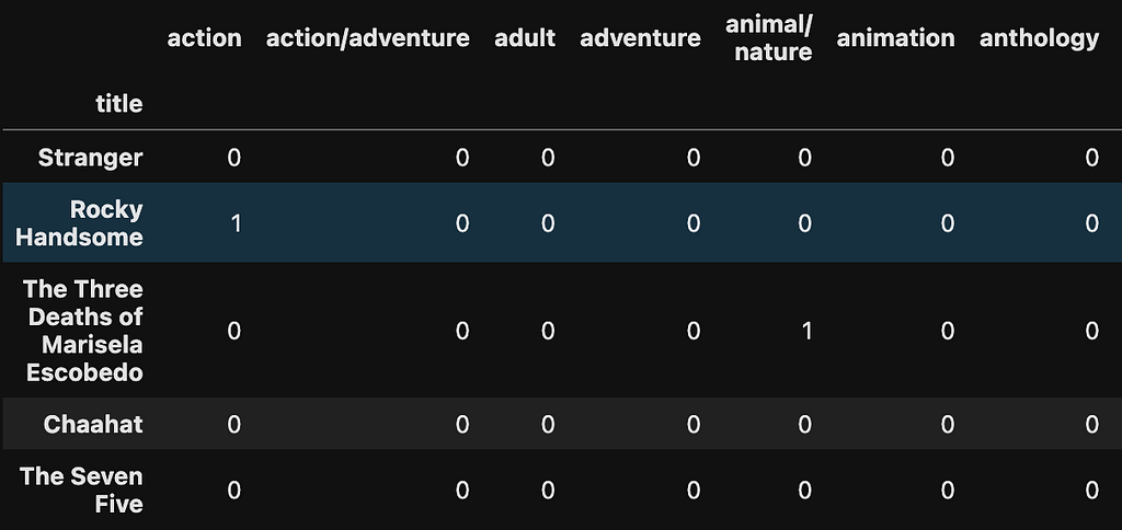
Now we turn the genre columns into dummy variables — each genre becomes its own column and if the movie or TV show is tagged with that genre then the column gets a 1, otherwise the value is 0.

# Combine genre columns into a single column
movies['all_genres'] = movies[['genre1', 'genre2', 'genre3']].astype(str).agg(','.join, axis=1)

# Split the genres and create dummy variables for each genre
genres = movies['all_genres'].str.get_dummies(sep=',')

# Concatenate the dummy variables with the original DataFrame
movies = pd.concat([movies, genres], axis=1)

# Drop unnecessary columns
movies.drop(['all_genres', 'genre1', 'genre2', 'genre3'], axis=1, inplace=True)

If we print the head of this DataFrame, this is what it looks like:

We need to use these dummy variables to build a matrix and run a similarity model across all pairs of movies:

# If there are duplicate columns due to the one-hot encoding, you can sum them up
movie_genre_matrix = movies.groupby(level=0, axis=1).sum()

# Calculate cosine similarity 
similarity_matrix = cosine_similarity(movie_genre_matrix, movie_genre_matrix)

Now we can define a function that calculates the most similar movies to a given title:

def find_similar_movies(movie_name, movie_genre_matrix, num_similar_movies=3):
    # Calculate cosine similarity
    similarity_matrix = cosine_similarity(movie_genre_matrix, movie_genre_matrix)
    
    # Find the index of the given movie
    movie_index = movie_genre_matrix.index.get_loc(movie_name)
    
    # Sort and get indices of most similar movies (excluding the movie itself)
    most_similar_indices = np.argsort(similarity_matrix[movie_index])[:-num_similar_movies-1:-1]
    
    # Return the most similar movies
    return movie_genre_matrix.index[most_similar_indices].tolist()

Let’s see if this model finds movies more similar to ‘Eat Pray Love,’ than the previous model:

# Example usage
similar_movies = find_similar_movies("Eat Pray Love", movie_genre_matrix, num_similar_movies=4)
print(similar_movies)

The output from this query, for me, were, ‘The Big Day’, ‘Love Dot Com: The Social Experiment’, and ’50 First Dates’. All of these movies are tagged as romantic comedies and dramas, just like Eat Pray Love.

‘Extremely Wicked, Shockingly Evil and Vile,’ the movie about a woman in love with Ted Bundy, is tagged with the genres romance, drama, and crime. The most similar movies are, ‘The Fury of a Patient Man’, ‘Much Loved’, and ‘Loving You’, all of which are also tagged with romance, drama, and crime. ‘Beavis and Butt-head Do America’ is tagged with the genres comedy, adventure and road trip. The most similar movies are ‘Pee-wee’s Big Holiday’, ‘A Shaun the Sheep Movie: Farmageddon’, and ‘The Secret Life of Pets 2.’ All of these movies are also tagged with the genres adventure and comedy — there are no other movies in this dataset (at least the portion I tagged) that match all three genres from Beavis and Butt-head.

Use the genre tags to create a network visualization

You can’t link data together without building a cool network visualization. There are a few ways to turn this data into a graph — we could look at how movies are conneted via genres, how genres are connected via movies, or a combination of the two. Because there are so many movies in this dataset, I just made a graph using genres as nodes and movies as edges.

Here is my code to turn the data into nodes and edges:

# Melt the dataframe to unpivot genre columns
melted_df = pd.melt(movies, id_vars=['title'], value_vars=['genre1', 'genre2', 'genre3'], var_name='Genre', value_name='GenreValue')

genre_links = pd.crosstab(index=melted_df['title'], columns=melted_df['GenreValue'])

# Create combinations of genres for each title
combinations_list = []

for title, group in melted_df.groupby('title')['GenreValue']:
    genre_combinations = list(combinations(group, 2))
    combinations_list.extend([(title, combo[0], combo[1]) for combo in genre_combinations])

# Create a new dataframe from the combinations list
combinations_df = pd.DataFrame(combinations_list, columns=['title', 'Genre1', 'Genre2'])

combinations_df = combinations_df[['Genre1','Genre2']]

combinations_df = combinations_df.rename(columns={"Genre1": "source", "Genre2": "target"}, errors="raise")

combinations_df = combinations_df.set_index('source')

combinations_df.to_csv("genreCombos.csv")

This produces a DataFrame that looks like this:

Each row in this DataFrame represents a movie that has been tagged with these two genres. We did not remove duplicates so there will be, presumably, many rows that look like row 1 above — there are many movies that are tagged as both romance and drama.

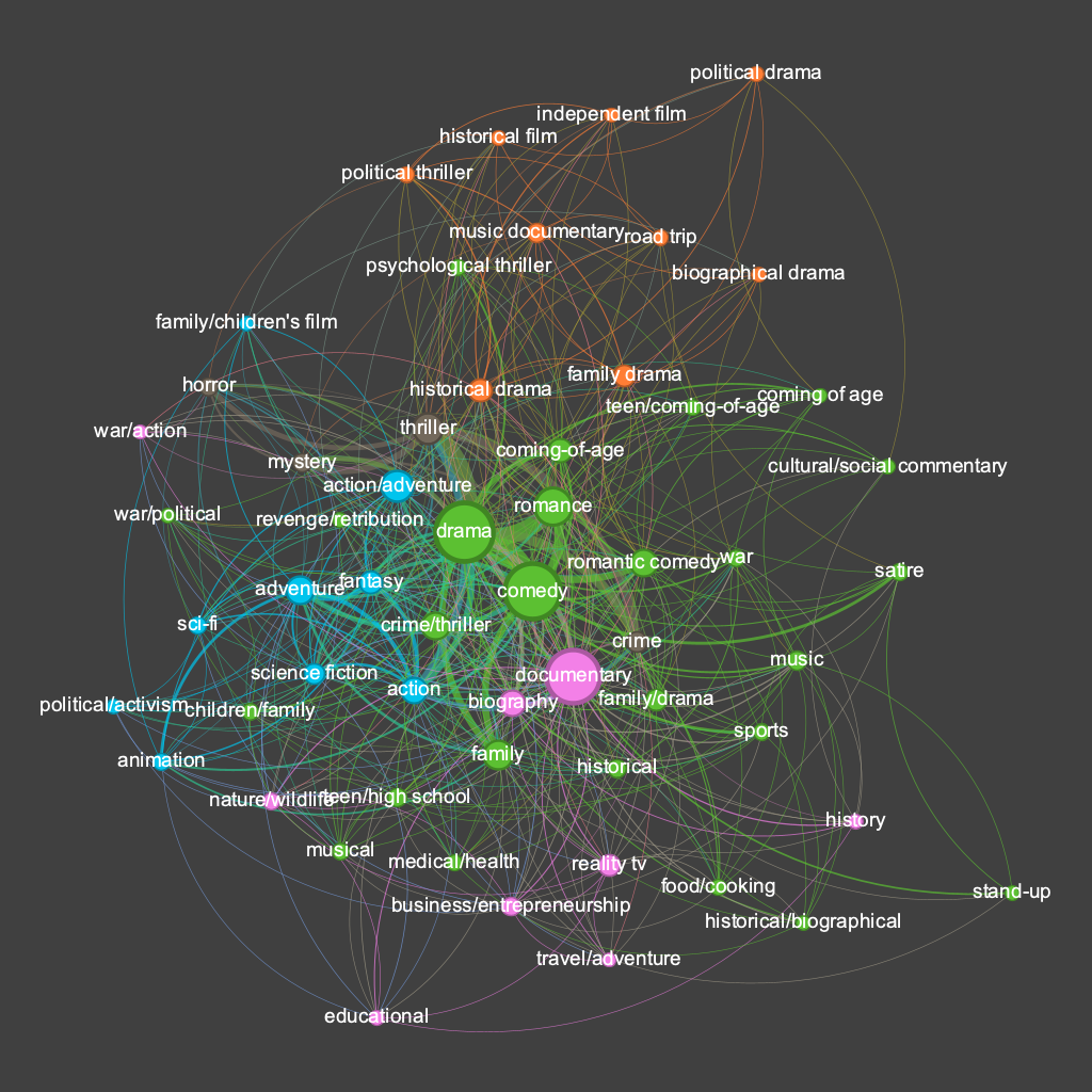
I used Gephi to build a visualization that looks like this:

The size of the nodes here represents the number of movies tagged with that genre. The color of the nodes is a function of a community detection algorithm — clusters that have closer connections amongst themselves than with nodes outside their cluster are colored the same.

This is fascinating to me. Drama, comedy, and documentary are the three largest nodes meaning more movies are tagged with those genres than any others. The genres also naturally form clusters that make intuitive sense. The genres most aligned with ‘documentary’ are colored pink and are mostly some kind of documentary sub-genre: nature/wildlife, reality TV, travel/adventure, history, educational, biography, etc. There are a core cluster of genres in green: drama, comedy, romance, coming of age, family, etc. One issue here is that we have multiple spellings of the ‘coming of age’ genre — a problem I would fix in future versions. There is a cluster in blue that includes action/adventure, fantasy, sci-fi, and animation. Again, we have duplicates and overlapping genres here which is a problem. There is also a small genre in brown that includes thriller, mystery, and horror — adult genres often present in the same film. The lack of connections between certain genres is also interesting — there are no films tagged with both ‘stand-up’ and ‘horror’, for example.

Conclusion

This project has shown me how even the most basic controlled vocabulary is useful, and potentially necessary, when building a content-based recommendation system. With just a list of genres we were able to tag movies and find other similar movies in a more explainable way than using just NLP. This could obviously be improved immensely through a more detailed and description genre taxonomy, but also through additional taxonomies including the cast and crew of films, the locations, etc.

As is usually the case when using LLMs, I was very impressed at first at how well it could perform this task, only to be disappointed when I viewed and tried to improve the results. Building taxonomies, ontologies, or any controlled vocabulary requires human engagement — there needs to be a human in the loop to ensure the vocabulary makes sense and will be useful in satisfying a particular use case.

LLMs and knowledge graphs (KGs) naturally fit together. One way they can be used together is that LLMs can help facilitate KG creation. LLMs can’t build a KG themselves but they can certainly help you create one.

Unraveling Unstructured Movie Data was originally published in Towards Data Science on Medium, where people are continuing the conversation by highlighting and responding to this story.