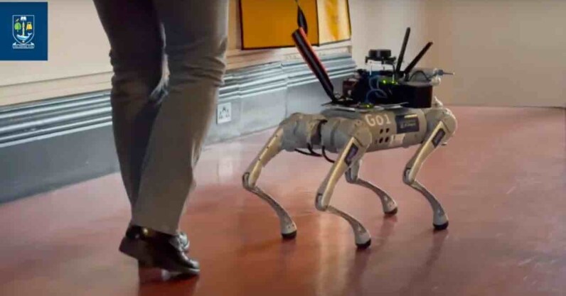
Automation doesn’t only threaten human workers. Our canine colleagues may also need new jobs because there’s a new robot guide dog in town — and it doesn’t even need walkies. Named Roboguide, the quadruped was bred at the University of Glasgow. The research team built the prototype pooch to support blind and partially sighted people in indoor spaces. Their design solves common problems in assistive tech. “One significant drawback of many current four-legged, two-legged and wheeled robots is that the technology which allows them to find their way around can limit their usefulness as assistants for the visually impaired,” said Dr Olaoluwa Popoola, the RoboGuide…
Python has become a language of choice, not just for developers but more and more businesses are relying on it as the backbone of their operations. Just what has contributed to the uncontested rise in its popularity and what career and salary prospects can Python developers expect in the future? Created in the 1990s by Guido van Rossum, who named it for the cult Monty Python’s Flying Circus, Python is a programming language that is relatively easy to pick up, as its syntax is straightforward and easy to read. This can mean it’s a good choice for beginners, but experienced…
On January 29, Amazon started inserting ads into the viewing experience of Prime Video subscribers. The company announced the change last year, telling customers that it will start showing “limited advertisements” with its service’s movies and shows so that it could invest “in compelling content and keep increasing that investment over a long period of time.” Those who don’t want to see ads will have to pay an extra fee of $3 a month. What it didn’t say, however, is that it’s also removing subscribers’ access to Dolby features if they choose to stay on the ad-supported tier. The change was first spotted by German tech publication 4kfilme and was confirmed by Forbes.
Forbes tested it out by streaming an episode of Jack Ryan, which was encoded with Dolby Vision high dynamic range video and Dolby Atmos sound on a TV that supports the technologies. The publication found that the boxes overlaid on top of the video confirming that Dolby Vision and Atmos are enabled were missing when they used an ad-supported account. Those boxes showed up as usual when played with an ad-free account.
That means customers will have to resort to paying the additional $3 a month on top of their subscription fee if they want to keep playing videos with Dolby Vision and Atmos enabled and if they don’t want their shows and movies interrupted by commercials. To note, Forbes also found that ad-free accounts still have access to HDR10+, which is a technology comparable to Dolby Vision.
Subscribers have been unhappy with the change, as expected, enough for a proposed class action lawsuit to be filed against the company in California federal court. The complaint accuses Amazon of violating consumer protection laws and calls its change of terms “deceptive” and “unfair.” It argues that those who’ve already paid for a year-long Prime subscription are expecting to enjoy an uninterrupted viewing experience as Amazon had promised. But since they’re also affected by this recent development, Amazon is “depriving them of the reasonable expectations to which they are entitled.” The class action is seeking at least $5 million in damages and is asking the court for an injunction “prohibiting [Amazon’s] deceptive conduct.”
This article originally appeared on Engadget at https://www.engadget.com/amazon-prime-video-wont-offer-dolby-vision-and-atmos-on-its-ad-supported-plan-093327322.html?src=rss
Evolution, visualisation, and applications of text embeddings
Image by DALL-E 3
As human beings, we can read and understand texts (at least some of them). Computers in opposite “think in numbers”, so they can’t automatically grasp the meaning of words and sentences. If we want computers to understand the natural language, we need to convert this information into the format that computers can work with — vectors of numbers.
People learned how to convert texts into machine-understandable format many years ago (one of the first versions was ASCII). Such an approach helps render and transfer texts but doesn’t encode the meaning of the words. At that time, the standard search technique was a keyword search when you were just looking for all the documents that contained specific words or N-grams.
Then, after decades, embeddings have emerged. We can calculate embeddings for words, sentences, and even images. Embeddings are also vectors of numbers, but they can capture the meaning. So, you can use them to do a semantic search and even work with documents in different languages.
In this article, I would like to dive deeper into the embedding topic and discuss all the details:
what preceded the embeddings and how they evolved,
how to calculate embeddings using OpenAI tools,
how to define whether sentences are close to each other,
how to visualise embeddings,
the most exciting part is how you could use embeddings in practice.
Let’s move on and learn about the evolution of embeddings.
Evolution of Embeddings
We will start our journey with a brief tour into the history of text representations.
Bag of Words
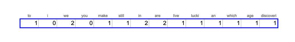
The most basic approach to converting texts into vectors is a bag of words. Let’s look at one of the famous quotes of Richard P. Feynman“We are lucky to live in an age in which we are still making discoveries”. We will use it to illustrate a bag of words approach.
The first step to get a bag of words vector is to split the text into words (tokens) and then reduce words to their base forms. For example, “running” will transform into “run”. This process is called stemming. We can use the NLTK Python package for it.
from nltk.stem import SnowballStemmer from nltk.tokenize import word_tokenize
text = 'We are lucky to live in an age in which we are still making discoveries'
# tokenization - splitting text into words words = word_tokenize(text) print(words) # ['We', 'are', 'lucky', 'to', 'live', 'in', 'an', 'age', 'in', 'which', # 'we', 'are', 'still', 'making', 'discoveries']
Actually, if we wanted to convert our text into a vector, we would have to take into account not only the words we have in the text but the whole vocabulary. Let’s assume we also have “i”, “you” and ”study” in our vocabulary and let’s create a vector from Feynman’s quote.
Graph by author
This approach is quite basic, and it doesn’t take into account the semantic meaning of the words, so the sentences “the girl is studying data science” and “the young woman is learning AI and ML” won’t be close to each other.
TF-IDF
A slightly improved version of the bag of the words approach is TF-IDF (Term Frequency — Inverse Document Frequency). It’s the multiplication of two metrics.
Term Frequency shows the frequency of the word in the document. The most common way to calculate it is to divide the raw count of the term in this document (like in the bag of words) by the total number of terms (words) in the document. However, there are many other approaches like just raw count, boolean “frequencies”, and different approaches to normalisation. You can learn more about different approaches on Wikipedia.
Inverse Document Frequency denotes how much information the word provides. For example, the words “a” or “that” don’t give you any additional information about the document’s topic. In contrast, words like “ChatGPT” or “bioinformatics” can help you define the domain (but not for this sentence). It’s calculated as the logarithm of the ratio of the total number of documents to those containing the word. The closer IDF is to 0 — the more common the word is and the less information it provides.
So, in the end, we will get vectors where common words (like “I” or “you”) will have low weights, while rare words that occur in the document multiple times will have higher weights. This strategy will give a bit better results, but it still can’t capture semantic meaning.
The other challenge with this approach is that it produces pretty sparse vectors. The length of the vectors is equal to the corpus size. There are about 470K unique words in English (source), so we will have huge vectors. Since the sentence won’t have more than 50 unique words, 99.99% of the values in vectors will be 0, not encoding any info. Looking at this, scientists started to think about dense vector representation.
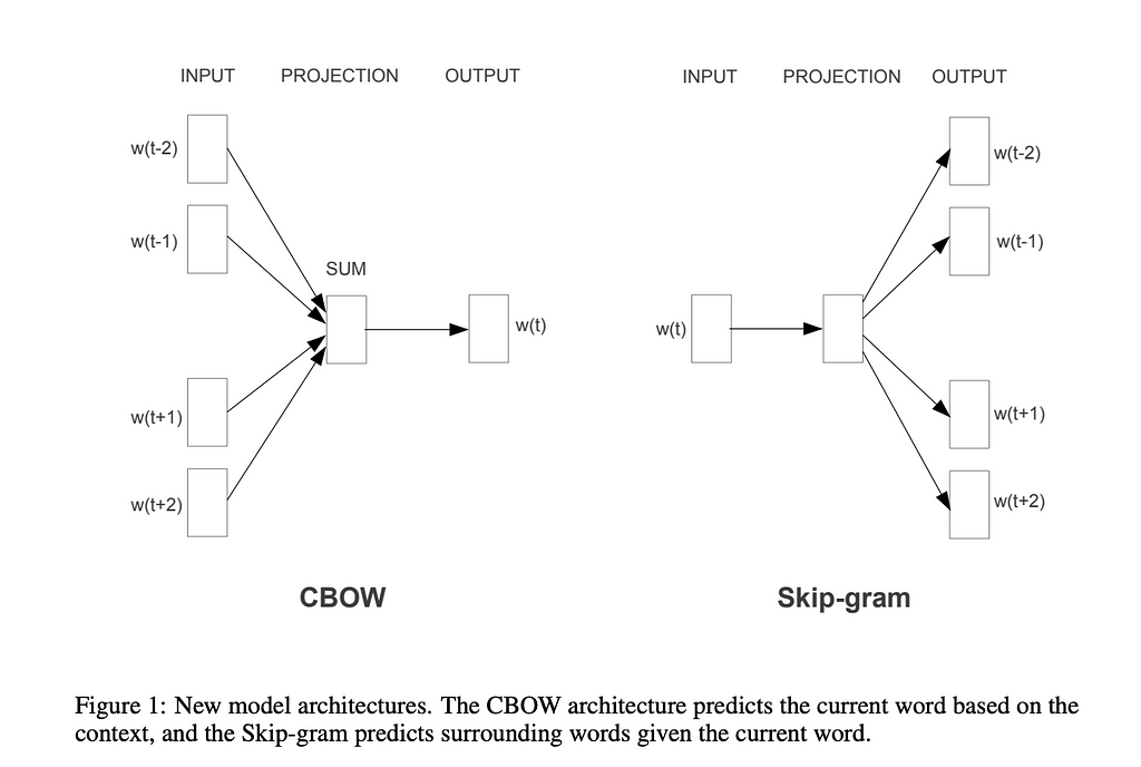
There are two different word2vec approaches mentioned in the paper: Continuous Bag of Words (when we predict the word based on the surrounding words) and Skip-gram (the opposite task — when we predict context based on the word).
Figure from the paper by Mikolov et al. 2013 | source
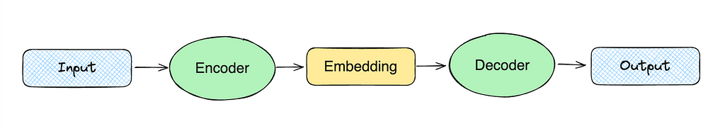
The high-level idea of dense vector representation is to train two models: encoder and decoder. For example, in the case of skip-gram, we might pass the word “christmas” to the encoder. Then, the encoder will produce a vector that we pass to the decoder expecting to get the words “merry”, “to”, and “you”.
Scheme by author
This model started to take into account the meaning of the words since it’s trained on the context of the words. However, it ignores morphology (information we can get from the word parts, for example, that “-less” means the lack of something). This drawback was addressed later by looking at subword skip-grams in GloVe.
Also, word2vec was capable of working only with words, but we would like to encode whole sentences. So, let’s move on to the next evolutional step with transformers.
Transformers and Sentence Embeddings
The next evolution was related to the transformers approach introduced in the “Attention Is All You Need” paper by Vaswani et al. Transformers were able to produce information-reach dense vectors and become the dominant technology for modern language models.
I won’t cover the details of the transformers’ architecture since it’s not so relevant to our topic and would take a lot of time. If you’re interested in learning more, there are a lot of materials about transformers, for example, “Transformers, Explained” or “The Illustrated Transformer”.
Transformers allow you to use the same “core” model and fine-tune it for different use cases without retraining the core model (which takes a lot of time and is quite costly). It led to the rise of pre-trained models. One of the first popular models was BERT (Bidirectional Encoder Representations from Transformers) by Google AI.
Internally, BERT still operates on a token level similar to word2vec, but we still want to get sentence embeddings. So, the naive approach could be to take an average of all tokens’ vectors. Unfortunately, this approach doesn’t show good performance.
This problem was solved in 2019 when Sentence-BERT was released. It outperformed all previous approaches to semantic textual similarity tasks and allowed the calculation of sentence embeddings.
It’s a huge topic so we won’t be able to cover it all in this article. So, if you’re really interested, you can learn more about the sentence embeddings in this article.
We’ve briefly covered the evolution of embeddings and got a high-level understanding of the theory. Now, it’s time to move on to practice and lear how to calculate embeddings using OpenAI tools.
Calculating embeddings
In this article, we will be using OpenAI embeddings. We will try a new model text-embedding-3-small that was released just recently. The new model shows better performance compared to text-embedding-ada-002:
The average score on a widely used multi-language retrieval (MIRACL) benchmark has risen from 31.4% to 44.0%.
The average performance on a frequently used benchmark for English tasks (MTEB) has also improved, rising from 61.0% to 62.3%.
OpenAI also released a new larger model text-embedding-3-large. Now, it’s their best performing embedding model.
As a data source, we will be working with a small sample of Stack Exchange Data Dump — an anonymised dump of all user-contributed content on the Stack Exchange network. I’ve selected a bunch of topics that look interesting to me and sample 100 questions from each of them. Topics range from Generative AI to coffee or bicycles so that we will see quite a wide variety of topics.
First, we need to calculate embeddings for all our Stack Exchange questions. It’s worth doing it once and storing results locally (in a file or vector storage). We can generate embeddings using the OpenAI Python package.
get_embedding("We are lucky to live in an age in which we are still making discoveries.")
As a result, we got a 1536-dimension vector of float numbers. We can now repeat it for all our data and start analysing the values.
The primary question you might have is how close the sentences are to each other by meaning. To uncover answers, let’s discuss the concept of distance between vectors.
Distance between vectors
Embeddings are actually vectors. So, if we want to understand how close two sentences are to each other, we can calculate the distance between vectors. A smaller distance would be equivalent to a closer semantic meaning.
Different metrics can be used to measure the distance between two vectors:
Euclidean distance (L2),
Manhattant distance (L1),
Dot product,
Cosine distance.
Let’s discuss them. As a simple example, we will be using two 2D vectors.
vector1 = [1, 4]
vector2 = [2, 2]
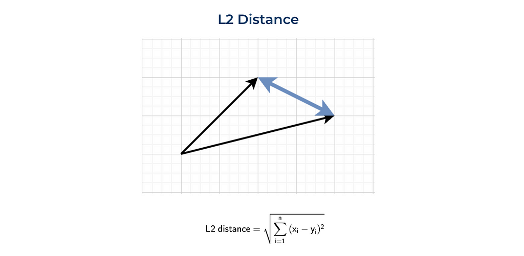
Euclidean distance (L2)
The most standard way to define distance between two points (or vectors) is Euclidean distance or L2 norm. This metric is the most commonly used in day-to-day life, for example, when we are talking about the distance between 2 towns.
Here’s a visual representation and formula for L2 distance.
Image by author
We can calculate this metric using vanilla Python or leveraging the numpy function.
np.linalg.norm((np.array(vector1) - np.array(vector2)), ord = 2) # 2.2361
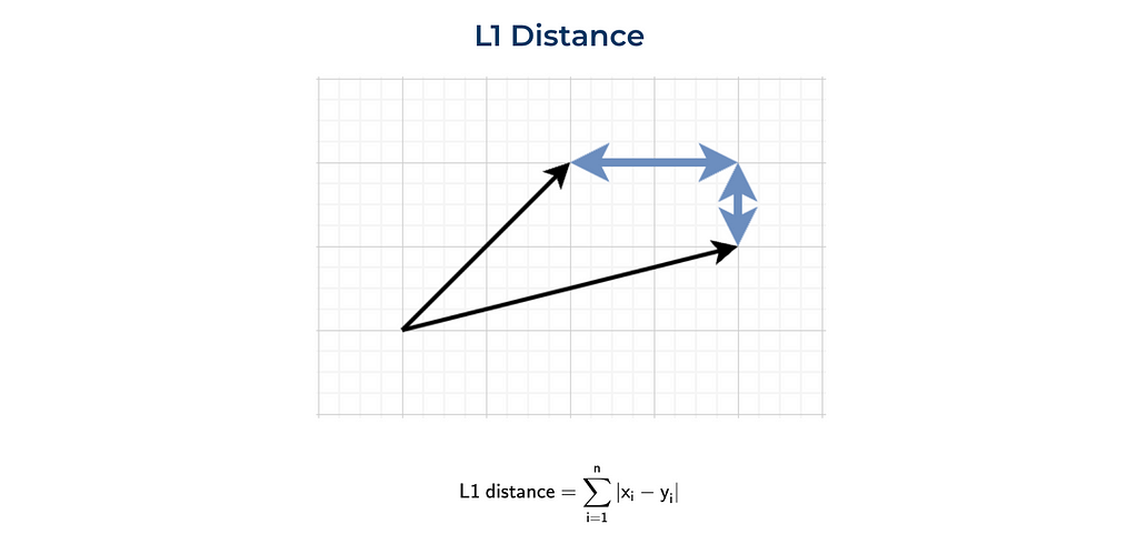
Manhattant distance (L1)
The other commonly used distance is the L1 norm or Manhattan distance. This distance was called after the island of Manhattan (New York). This island has a grid layout of streets, and the shortest routes between two points in Manhattan will be L1 distance since you need to follow the grid.
Image by author
We can also implement it from scratch or use the numpy function.
This metric is a bit tricky to interpret. On the one hand, it shows you whether vectors are pointing in one direction. On the other hand, the results highly depend on the magnitudes of the vectors. For example, let’s calculate the dot products between two pairs of vectors:
(1, 1) vs (1, 1)
(1, 1) vs (10, 10).
In both cases, vectors are collinear, but the dot product is ten times bigger in the second case: 2 vs 20.
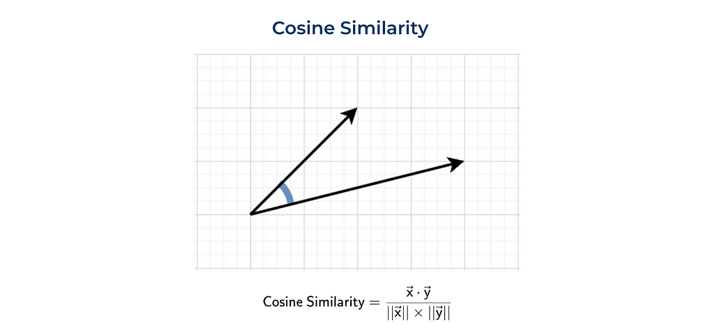
Cosine similarity
Quite often, cosine similarity is used. Cosine similarity is a dot product normalised by vectors’ magnitudes (or normes).
Image by author
We can either calculate everything ourselves (as previously) or use the function from sklearn.
The function cosine_similarity expects 2D arrays. That’s why we need to reshape the numpy arrays.
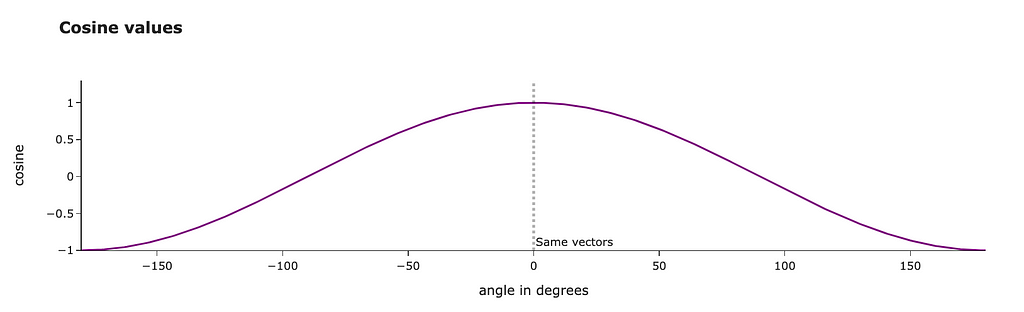
Let’s talk a bit about the physical meaning of this metric. Cosine similarity is equal to the cosine between two vectors. The closer the vectors are, the higher the metric value.
Image by author
We can even calculate the exact angle between our vectors in degrees. We get results around 30 degrees, and it looks pretty reasonable.
import math
math.degrees(math.acos(0.8575))

# 30.96
What metric to use?
We’ve discussed different ways to calculate the distance between two vectors, and you might start thinking about which one to use.
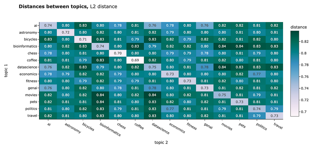
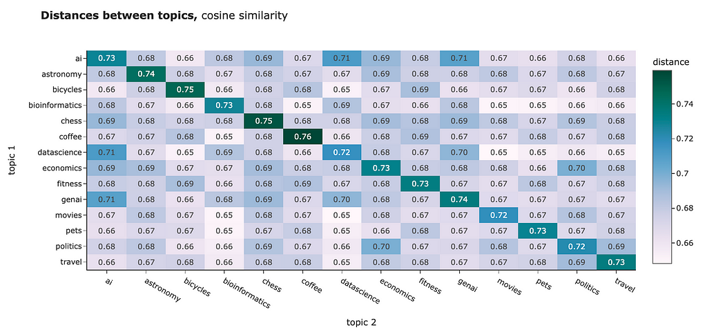
You can use any distance to compare the embeddings you have. For example, I calculated the average distances between the different clusters. Both L2 distance and cosine similarity show us similar pictures:
Objects within a cluster are closer to each other than to other clusters. It’s a bit tricky to interpret our results since for L2 distance, closer means lower distance, while for cosine similarity — the metric is higher for closer objects. Don’t get confused.
We can spot that some topics are really close to each other, for example, “politics” and “economics” or “ai” and “datascience”.
Image by authorImage by author
However, for NLP tasks, the best practice is usually to use cosine similarity. Some reasons behind it:
Cosine similarity is between -1 and 1, while L1 and L2 are unbounded, so it’s easier to interpret.
From the practical perspective, it’s more effective to calculate dot products than square roots for Euclidean distance.
Cosine similarity is less affected by the curse of dimensionality (we will talk about it in a second).
OpenAI embeddings are already normed, so dot product and cosine similarity are equal in this case.
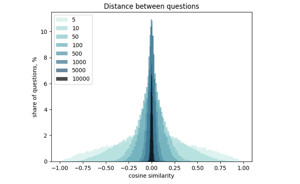
You might spot in the results above that the difference between inter- and intra-cluster distances is not so big. The root cause is the high dimensionality of our vectors. This effect is called “the curse of dimensionality”: the higher the dimension, the narrower the distribution of distances between vectors. You can learn more details about it in this article.
I would like to briefly show you how it works so that you get some intuition. I calculated a distribution of OpenAI embedding values and generated sets of 300 vectors with different dimensionalities. Then, I calculated the distances between all the vectors and draw a histogram. You can easily see that the increase in vector dimensionality makes the distribution narrower.
Graph by author
We’ve learned how to measure the similarities between the embeddings. With that we’ve finished with a theoretical part and moving to more practical part (visualisations and practical applications). Let’s start with visualisations since it’s always better to see your data first.
Visualising embeddings
The best way to understand the data is to visualise it. Unfortunately, embeddings have 1536 dimensions, so it’s pretty challenging to look at the data. However, there’s a way: we could use dimensionality reduction techniques to project vectors in two-dimensional space.
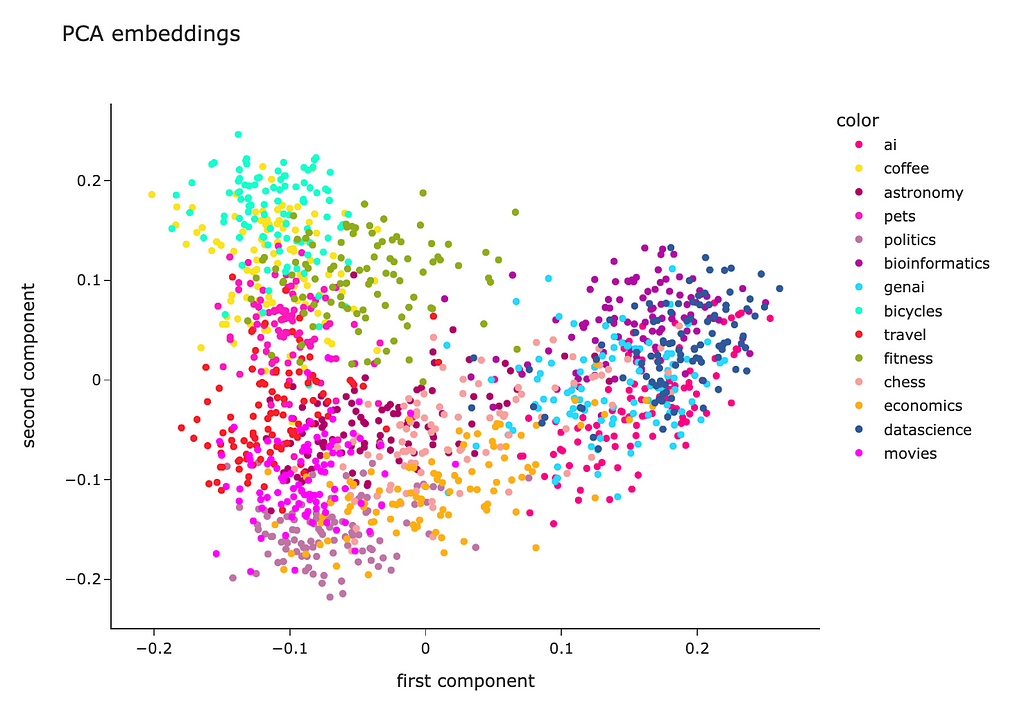
PCA
The most basic dimensionality reduction technique is PCA (Principal Component Analysis). Let’s try to use it.
First, we need to convert our embeddings into a 2D numpy array to pass it to sklearn.
Then, we need to initialise a PCA model with n_components = 2 (because we want to create a 2D visualisation), train the model on the whole data and predict new values.
We can see that questions from each topic are pretty close to each other, which is good. However, all the clusters are mixed, so there’s room for improvement.
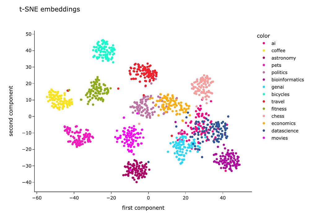
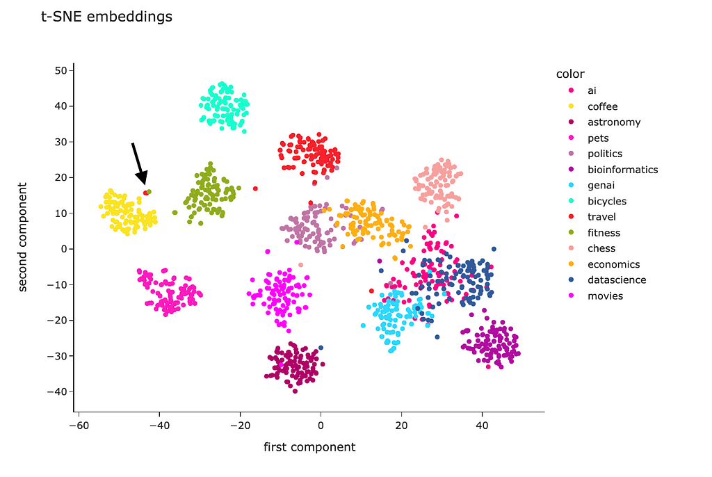
t-SNE
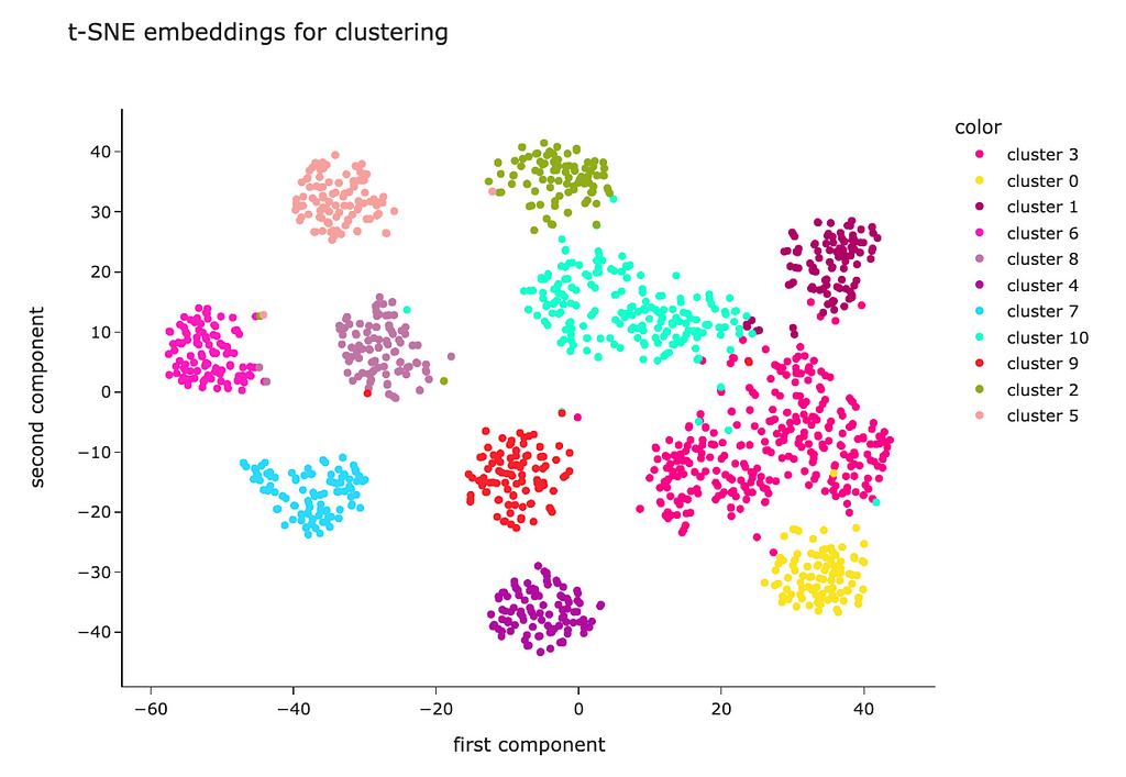
PCA is a linear algorithm, while most of the relations are non-linear in real life. So, we may not be able to separate the clusters because of non-linearity. Let’s try to use a non-linear algorithm t-SNE and see whether it will be able to show better results.
The code is almost identical. I just used the t-SNE model instead of PCA.
The t-SNE result looks way better. Most of the clusters are separated except “genai”, “datascience” and “ai”. However, it’s pretty expected — I doubt I could separate these topics myself.
Looking at this visualisation, we see that embeddings are pretty good at encoding semantic meaning.
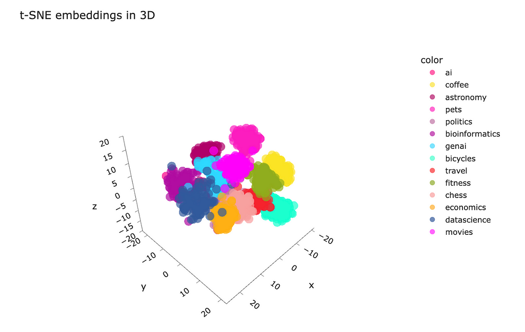
Also, you can make a projection to three-dimensional space and visualise it. I’m not sure whether it would be practical, but it can be insightful and engaging to play with the data in 3D.
fig = px.scatter_3d( x = tsne_3d_embeddings_values[:,0], y = tsne_3d_embeddings_values[:,1], z = tsne_3d_embeddings_values[:,2], color = df.topic.values, hover_name = df.full_text.values, title = 't-SNE embeddings', width = 800, height = 600, color_discrete_sequence = plotly.colors.qualitative.Alphabet_r, opacity = 0.7 ) fig.update_layout(xaxis_title = 'first component', yaxis_title = 'second component') fig.show()
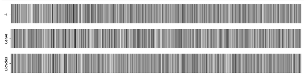
Barcodes
The way to understand the embeddings is to visualise a couple of them as bar codes and see the correlations. I picked three examples of embeddings: two are closest to each other, and the other is the farthest example in our dataset.
It’s not easy to see whether vectors are close to each other in our case because of high dimensionality. However, I still like this visualisation. It might be helpful in some cases, so I am sharing this idea with you.
We’ve learned how to visualise embeddings and have no doubts left about their ability to grasp the meaning of the text. Now, it’s time to move on to the most interesting and fascinating part and discuss how you can leverage embeddings in practice.
Practical applications
Of course, embeddings’ primary goal is not to encode texts as vectors of numbers or visualise them just for the sake of it. We can benefit a lot from our ability to capture the texts’ meanings. Let’s go through a bunch of more practical examples.
Clustering
Let’s start with clustering. Clustering is an unsupervised learning technique that allows you to split your data into groups without any initial labels. Clustering can help you understand the internal structural patterns in your data.
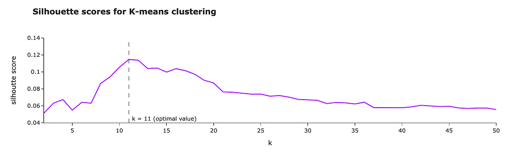
We will use one of the most basic clustering algorithms — K-means. For the K-means algorithm, we need to specify the number of clusters. We can define the optimal number of clusters using silhouette scores.
Let’s try k (number of clusters) between 2 and 50. For each k, we will train a model and calculate silhouette scores. The higher silhouette score — the better clustering we got.
from sklearn.cluster import KMeans from sklearn.metrics import silhouette_score import tqdm
silhouette_scores = [] for k in tqdm.tqdm(range(2, 51)): kmeans = KMeans(n_clusters=k, random_state=42, n_init = 'auto').fit(embeddings_array) kmeans_labels = kmeans.labels_ silhouette_scores.append( { 'k': k, 'silhouette_score': silhouette_score(embeddings_array, kmeans_labels, metric = 'cosine') } )
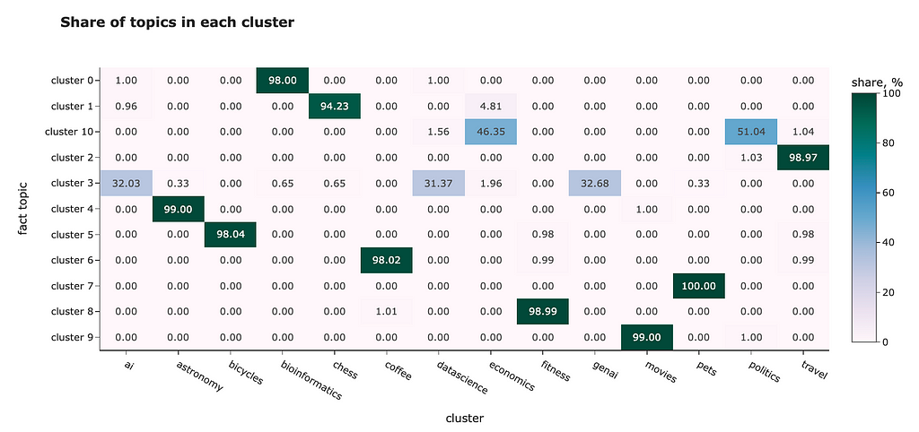
fig = px.imshow( cluster_stats_df.values, x = cluster_stats_df.columns, y = cluster_stats_df.index, text_auto = '.2f', aspect = "auto", labels=dict(x="cluster", y="fact topic", color="share, %"), color_continuous_scale='pubugn', title = '<b>Share of topics in each cluster</b>', height = 550)
fig.show()
In most cases, clusterisation worked perfectly. For example, cluster 5 contains almost only questions about bicycles, while cluster 6 is about coffee. However, it wasn’t able to distinguish close topics:
“ai”, “genai” and “datascience” are all in one cluster,
the same store with “economics” and “politics”.
We used only embeddings as the features in this example, but if you have any additional information (for example, age, gender or country of the user who asked the question), you can include it in the model, too.
Classification
We can use embeddings for classification or regression tasks. For example, you can do it to predict customer reviews’ sentiment (classification) or NPS score (regression).
Since classification and regression are supervised learning, you will need to have labels. Luckily, we know the topics for our questions and can fit a model to predict them.
I will use a Random Forest Classifier. If you need a quick refresher about Random Forests, you can find it here. To assess the classification model’s performance correctly, we will split our dataset into train and test sets (80% vs 20%). Then, we can train our model on a train set and measure the quality on a test set (questions that the model hasn’t seen before).
from sklearn.ensemble import RandomForestClassifier
from sklearn.model_selection import train_test_split
class_model = RandomForestClassifier(max_depth = 10)

# defining features and target
X = embeddings_array
y = df.topic

# splitting data into train and test sets
X_train, X_test, y_train, y_test = train_test_split(
    X, y, random_state = 42, test_size=0.2, stratify=y
)

# fit & predict
class_model.fit(X_train, y_train)
y_pred = class_model.predict(X_test)
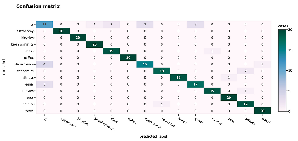
To estimate the model’s performance, let’s calculate a confusion matrix. In an ideal situation, all non-diagonal elements should be 0.
from sklearn.metrics import confusion_matrix
cm = confusion_matrix(y_test, y_pred)

fig = px.imshow(
  cm, x = class_model.classes_,
  y = class_model.classes_, text_auto='d',
  aspect="auto",
  labels=dict(
      x="predicted label", y="true label",
      color="cases"),
  color_continuous_scale='pubugn',
  title = '<b>Confusion matrix</b>', height = 550)

fig.show()
We can see similar results to clusterisation: some topics are easy to classify, and accuracy is 100%, for example, “bicycles” or “travel”, while some others are difficult to distinguish (especially “ai”).
However, we achieved 91.8% overall accuracy, which is quite good.
Finding anomalies
We can also use embedding to find anomalies in our data. For example, at the t-SNE graph, we saw that some questions are pretty far from their clusters, for instance, for the “travel” topic. Let’s look at this theme and try to find anomalies. We will use the Isolation Forest algorithm for it.
So, here we are. We’ve found the most uncommon comment for the travel topic (source).
Is it safe to drink the water from the fountains found all over
the older parts of Rome?

When I visited Rome and walked around the older sections, I saw many
different types of fountains that were constantly running with water.
Some went into the ground, some collected in basins, etc.

Is the water coming out of these fountains potable? Safe for visitors
to drink from? Any etiquette regarding their use that a visitor
should know about?
Since it talks about water, the embedding of this comment is close to the coffee topic where people also discuss water to pour coffee. So, the embedding representation is quite reasonable.
We could find it on our t-SNE visualisation and see that it’s actually close to the coffee cluster.
Graph by author
RAG — Retrieval Augmented Generation
With the recently increased popularity of LLMs, embeddings have been broadly used in RAG use cases.
We need Retrieval Augmented Generation when we have a lot of documents (for example, all the questions from Stack Exchange), and we can’t pass them all to an LLM because
LLMs have limits on the context size (right now, it’s 128K for GPT-4 Turbo).
We pay for tokens, so it’s more expensive to pass all the information all the time.
To be able to work with an extensive knowledge base, we can leverage the RAG approach:
Compute embeddings for all the documents and store them in vector storage.
When we get a user request, we can calculate its embedding and retrieve relevant documents from the storage for this request.
Pass only relevant documents to LLM to get a final answer.
To learn more about RAG, don’t hesitate to read my article with much more details here.
Summary
In this article, we’ve discussed text embeddings in much detail. Hopefully, now you have a complete and deep understanding of this topic. Here’s a quick recap of our journey:
Firstly, we went through the evolution of approaches to work with texts.
Then, we discussed how to understand whether texts have similar meanings to each other.
After that, we saw different approaches to text embedding visualisation.
Finally, we tried to use embeddings as features in different practical tasks such as clustering, classification, anomaly detection and RAG.
Thank you a lot for reading this article. If you have any follow-up questions or comments, please leave them in the comments section.
Connections is the new puzzle game from the New York Times, and it can be quite difficult. If you need a hand with solving today’s puzzle, we’re here to help.
We use cookies on our website to give you the most relevant experience by remembering your preferences and repeat visits. By clicking “Accept”, you consent to the use of ALL the cookies.
This website uses cookies to improve your experience while you navigate through the website. Out of these, the cookies that are categorized as necessary are stored on your browser as they are essential for the working of basic functionalities of the website. We also use third-party cookies that help us analyze and understand how you use this website. These cookies will be stored in your browser only with your consent. You also have the option to opt-out of these cookies. But opting out of some of these cookies may affect your browsing experience.
Necessary cookies are absolutely essential for the website to function properly. These cookies ensure basic functionalities and security features of the website, anonymously.
Cookie
Duration
Description
cookielawinfo-checkbox-analytics
11 months
This cookie is set by GDPR Cookie Consent plugin. The cookie is used to store the user consent for the cookies in the category "Analytics".
cookielawinfo-checkbox-functional
11 months
The cookie is set by GDPR cookie consent to record the user consent for the cookies in the category "Functional".
cookielawinfo-checkbox-necessary
11 months
This cookie is set by GDPR Cookie Consent plugin. The cookies is used to store the user consent for the cookies in the category "Necessary".
cookielawinfo-checkbox-others
11 months
This cookie is set by GDPR Cookie Consent plugin. The cookie is used to store the user consent for the cookies in the category "Other.
cookielawinfo-checkbox-performance
11 months
This cookie is set by GDPR Cookie Consent plugin. The cookie is used to store the user consent for the cookies in the category "Performance".
viewed_cookie_policy
11 months
The cookie is set by the GDPR Cookie Consent plugin and is used to store whether or not user has consented to the use of cookies. It does not store any personal data.
Functional cookies help to perform certain functionalities like sharing the content of the website on social media platforms, collect feedbacks, and other third-party features.
Performance cookies are used to understand and analyze the key performance indexes of the website which helps in delivering a better user experience for the visitors.
Analytical cookies are used to understand how visitors interact with the website. These cookies help provide information on metrics the number of visitors, bounce rate, traffic source, etc.
Advertisement cookies are used to provide visitors with relevant ads and marketing campaigns. These cookies track visitors across websites and collect information to provide customized ads.