Volkswagen reveals its ID.7 Tourer model, one of the first electric estate cars with a huge luggage compartment and an electric range of up to 425 miles in select models.
The advanced RAG paradigm comprises of a set of techniques targeted at addressing known limitations of naive RAG. This article first discusses these techniques, which can be categorized into pre-retrieval, retrieval, and post-retrieval optimizations.
In the second half, you will learn how to implement a naive RAG pipeline using Llamaindex in Python, which will then be enhanced to an advanced RAG pipeline with a selection of the following advanced RAG techniques:
This article focuses on the advanced RAG paradigm and its implementation. If you are unfamiliar with the fundamentals of RAG, you can catch up on it here:
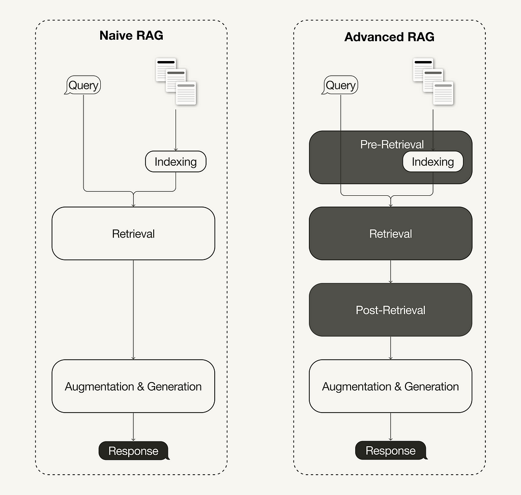
With the recent advancements in the RAG domain, advanced RAG has evolved as a new paradigm with targeted enhancements to address some of the limitations of the naive RAG paradigm. As summarized in a recent survey [1], advanced RAG techniques can be categorized into pre-retrieval, retrieval, and post-retrieval optimizations.
Difference between Naive and Advanced RAG (Image by the author, inspired by [1])
Pre-retrieval optimization
Pre-retrieval optimizations focus on data indexing optimizations as well as query optimizations. Data indexing optimization techniques aim to store the data in a way that helps you improve retrieval efficiency, such as [1]:
Sliding window uses an overlap between chunks and is one of the simplest techniques.
Enhancing data granularity applies data cleaning techniques, such as removing irrelevant information, confirming factual accuracy, updating outdated information, etc.
Adding metadata, such as dates, purposes, or chapters, for filtering purposes.
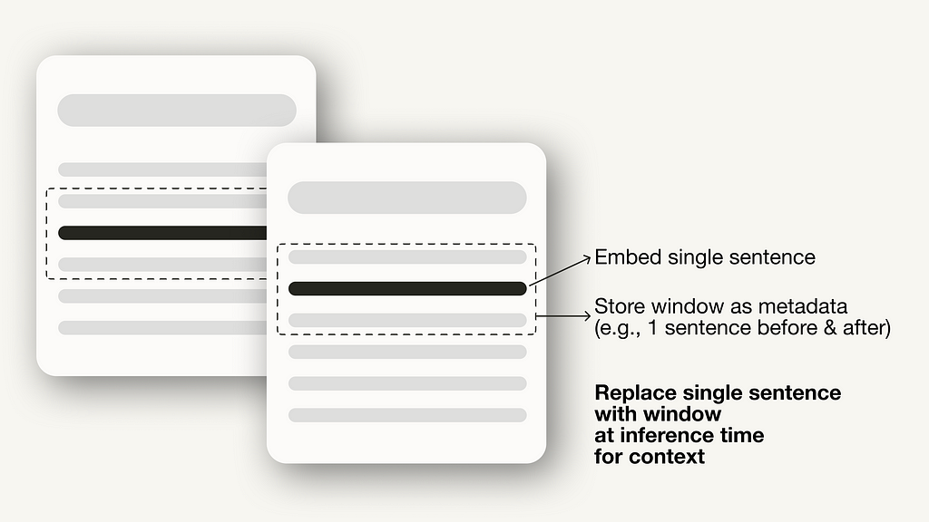
Optimizing index structures involves different strategies to index data, such as adjusting the chunk sizes or using multi-indexing strategies. One technique we will implement in this article is sentence window retrieval, which embeds single sentences for retrieval and replaces them with a larger text window at inference time.
Sentence window retrieval
Additionally, pre-retrieval techniques aren’t limited to data indexing and can cover techniques at inference time, such as query routing, query rewriting, and query expansion.
Retrieval optimization
The retrieval stage aims to identify the most relevant context. Usually, the retrieval is based on vector search, which calculates the semantic similarity between the query and the indexed data. Thus, the majority of retrieval optimization techniques revolve around the embedding models [1]:
Fine-tuning embedding models customizes embedding models to domain-specific contexts, especially for domains with evolving or rare terms. For example, BAAI/bge-small-en is a high-performance embedding model that can be fine-tuned (see Fine-tuning guide)
Dynamic Embedding adapts to the context in which words are used, unlike static embedding, which uses a single vector for each word. For example, OpenAI’s embeddings-ada-02 is a sophisticated dynamic embedding model that captures contextual understanding. [1]
There are also other retrieval techniques besides vector search, such as hybrid search, which often refers to the concept of combining vector search with keyword-based search. This retrieval technique is beneficial if your retrieval requires exact keyword matches.
Additional processing of the retrieved context can help address issues such as exceeding the context window limit or introducing noise, thus hindering the focus on crucial information. Post-retrieval optimization techniques summarized in the RAG survey [1] are:
Prompt compression reduces the overall prompt length by removing irrelevant and highlighting important context.
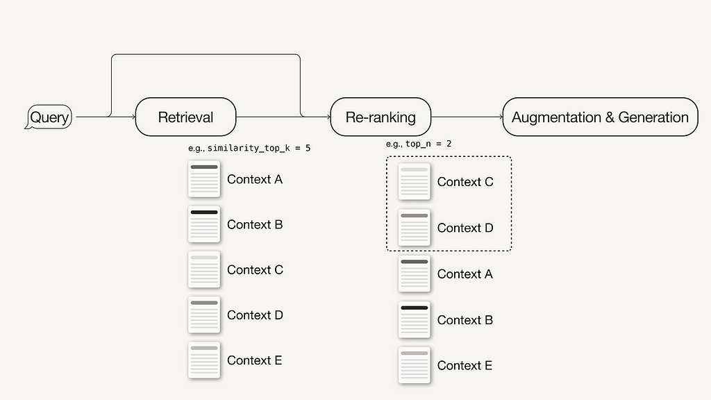
Re-ranking uses machine learning models to recalculate the relevance scores of the retrieved contexts.
Re-ranking
For additional ideas on how to improve the performance of your RAG pipeline to make it production-ready, continue reading here:
This section discusses the required packages and API keys to follow along in this article.
Required Packages
This article will guide you through implementing a naive and an advanced RAG pipeline using LlamaIndex in Python.
pip install llama-index
In this article, we will be using LlamaIndex v0.10. If you are upgrading from an older LlamaIndex version, you need to run the following commands to install and run LlamaIndex properly:
LlamaIndex offers an option to store vector embeddings locally in JSON files for persistent storage, which is great for quickly prototyping an idea. However, we will use a vector database for persistent storage since advanced RAG techniques aim for production-ready applications.
Since we will need metadata storage and hybrid search capabilities in addition to storing the vector embeddings, we will use the open source vector database Weaviate (v3.26.2), which supports these features.
We will be using Weaviate embedded, which you can use for free without registering for an API key. However, this tutorial uses an embedding model and LLM from OpenAI, for which you will need an OpenAI API key. To obtain one, you need an OpenAI account and then “Create new secret key” under API keys.
Next, create a local .env file in your root directory and define your API keys in it:
OPENAI_API_KEY="<YOUR_OPENAI_API_KEY>"
Afterwards, you can load your API keys with the following code:
# !pip install python-dotenv
import os
from dotenv import load_dotenv,find_dotenv

load_dotenv(find_dotenv())
Implementing Naive RAG with LlamaIndex
This section discusses how to implement a naive RAG pipeline using LlamaIndex. You can find the entire naive RAG pipeline in this Jupyter Notebook. For the implementation using LangChain, you can continue in this article (naive RAG pipeline using LangChain).
Step 1: Define the embedding model and LLM
First, you can define an embedding model and LLM in a global settings object. Doing this means you don’t have to specify the models explicitly in the code again.
Embedding model: used to generate vector embeddings for the document chunks and the query.
LLM: used to generate an answer based on the user query and the relevant context.
from llama_index.embeddings.openai import OpenAIEmbedding from llama_index.llms.openai import OpenAI from llama_index.core.settings import Settings
Next, you will create a local directory named data in your root directory and download some example data from the LlamaIndex GitHub repository (MIT license).
Afterward, you can load the data for further processing:
from llama_index.core import SimpleDirectoryReader

# Load data
documents = SimpleDirectoryReader(
        input_files=["./data/paul_graham_essay.txt"]
).load_data()
Step 3: Chunk documents into nodes
As the entire document is too large to fit into the context window of the LLM, you will need to partition it into smaller text chunks, which are called Nodes in LlamaIndex. You can parse the loaded documents into nodes using the SimpleNodeParser with a defined chunk size of 1024.
from llama_index.core.node_parser import SimpleNodeParser
# Extract nodes from documents nodes = node_parser.get_nodes_from_documents(documents)
Step 4: Build index
Next, you will build the index that stores all the external knowledge in Weaviate, an open source vector database.
First, you will need to connect to a Weaviate instance. In this case, we’re using Weaviate Embedded, which allows you to experiment in Notebooks for free without an API key. For a production-ready solution, deploying Weaviate yourself, e.g., via Docker or utilizing a managed service, is recommended.
import weaviate

# Connect to your Weaviate instance
client = weaviate.Client(
    embedded_options=weaviate.embedded.EmbeddedOptions(),
)
Next, you will build a VectorStoreIndex from the Weaviate client to store your data in and interact with.
from llama_index.core import VectorStoreIndex, StorageContext from llama_index.vector_stores.weaviate import WeaviateVectorStore
# Set up the storage for the embeddings storage_context = StorageContext.from_defaults(vector_store=vector_store)
# Setup the index # build VectorStoreIndex that takes care of chunking documents # and encoding chunks to embeddings for future retrieval index = VectorStoreIndex( nodes, storage_context = storage_context, )
Step 5: Setup query engine
Lastly, you will set up the index as the query engine.
# The QueryEngine class is equipped with the generator
# and facilitates the retrieval and generation steps
query_engine = index.as_query_engine()
Step 6: Run a naive RAG query on your data
Now, you can run a naive RAG query on your data, as shown below:
# Run your naive RAG query
response = query_engine.query(
    "What happened at Interleaf?"
)
Implementing Advanced RAG with LlamaIndex
In this section, we will cover some simple adjustments you can make to turn the above naive RAG pipeline into an advanced one. This walkthrough will cover the following selection of advanced RAG techniques:
For the sentence window retrieval technique, you need to make two adjustments: First, you must adjust how you store and post-process your data. Instead of the SimpleNodeParser, we will use the SentenceWindowNodeParser.
from llama_index.core.node_parser import SentenceWindowNodeParser
It separates the document into single sentences, which will be embedded.
For each sentence, it creates a context window. If you specify a window_size = 3, the resulting window will be three sentences long, starting at the previous sentence of the embedded sentence and spanning the sentence after. The window will be stored as metadata.
During retrieval, the sentence that most closely matches the query is returned. After retrieval, you need to replace the sentence with the entire window from the metadata by defining a MetadataReplacementPostProcessor and using it in the list of node_postprocessors.
from llama_index.core.postprocessor import MetadataReplacementPostProcessor
# The target key defaults to `window` to match the node_parser's default postproc = MetadataReplacementPostProcessor( target_metadata_key="window" )
Implementing a hybrid search in LlamaIndex is as easy as two parameter changes to the query_engine if the underlying vector database supports hybrid search queries. The alpha parameter specifies the weighting between vector search and keyword-based search, where alpha=0 means keyword-based search and alpha=1 means pure vector search.
There are many more different techniques within the advanced RAG paradigm. If you are interested in further implementations, I recommend the following two resources:
This article covered the concept of advanced RAG, which covers a set of techniques to address the limitations of the naive RAG paradigm. After an overview of advanced RAG techniques, which can be categorized into pre-retrieval, retrieval, and post-retrieval techniques, this article implemented a naive and advanced RAG pipeline using LlamaIndex for orchestration.
The RAG pipeline components were language models from OpenAI, a reranker model from BAAI hosted on Hugging Face, and a Weaviate vector database.
We implemented the following selection of techniques using LlamaIndex in Python:
I am a Developer Advocate at Weaviate at the time of this writing.
References
Literature
[1] Gao, Y., Xiong, Y., Gao, X., Jia, K., Pan, J., Bi, Y., … & Wang, H. (2023). Retrieval-augmented generation for large language models: A survey. arXiv preprint arXiv:2312.10997.
Images
If not otherwise stated, all images are created by the author.
Decoding the Math behind Reinforcement Learning, introducing the RL Framework, and building one RL simulation from scratch in Python.
Image generated by DALL-E
Reinforcement learning (RL) stands as a pivotal element in the landscape of artificial intelligence, known for its unique method of teaching machines to make decisions through their own experiences within an environment. In this article, we’re going to take a deep dive into what makes RL tick. We’ll break down its core concepts, highlight the broad range of its applications, decode the math, and guide you through building it from scratch.
Reinforcement learning, or RL, is an area of artificial intelligence that’s all about teaching machines to make smart choices. Think of it as similar to training a dog. You give treats to encourage the behaviors you like, and over time, the dog — or in this case, a computer program — figures out which actions get the best results. But instead of yummy treats, we use numerical rewards, and the machine’s goal is to score as high as it can.
Now, your dog might not be a champ at board games, but RL can outsmart world champions. Take the time Google’s DeepMind introduced AlphaGo. This RL-powered software went head-to-head with Lee Sedol, a top player in the game Go, and won back in 2016. AlphaGo got better by playing loads of games against both human and computer opponents, learning and improving with each game.
But RL isn’t just for beating game champions. It’s also making waves in robotics, helping robots learn tasks that are tough to code directly, like grabbing and moving objects. And it’s behind the personalized recommendations you get on platforms like Netflix and Spotify, tweaking its suggestions to match what you like.
How does it work?
At the core of reinforcement learning (RL) is this dynamic between an agent (that’s you or the algorithm) and its environment. Picture this: you’re playing a video game. You’re the agent, the game’s world is the environment, and your mission is to rack up as many points as possible. Every moment in the game is a chance to make a move, and depending on what you do, the game throws back a new scenario and maybe some rewards (like points for snagging a coin or knocking out an enemy).
This give-and-take keeps going, with the agent (whether it’s you or the algorithm) figuring out which moves bring in the most rewards as time goes on. It’s all about trial and error, where the machine slowly but surely uncovers the best game plan, or policy, to hit its targets.
RL is a bit different from other ways of learning machines, like supervised learning, where a model learns from a set of data that already has the right answers, or unsupervised learning, which is all about spotting patterns in data without clear-cut instructions. With RL, there’s no cheat sheet. The agent learns purely through its adventures — making choices, seeing what happens, and learning from it.
This article is just the beginning of our “Reinforcement Learning 101” series. We’re going to break down the essentials of reinforcement learning, from the basic ideas to the intricate algorithms that power some of the most sophisticated AI out there. And here’s the fun part: you’ll get to try your hand at coding these concepts in Python, starting with our very first article. So, whether you’re a student, a developer, or just someone fascinated by AI, this series will give you the tools and knowledge to dive into the thrilling realm of reinforcement learning.
Let’s get started!
The RL Framework
Let’s dive deeper into the heart of reinforcement learning, where everything revolves around the interaction between an agent and its environment. This relationship is all about a cycle of actions, states, and rewards, helping the agent learn the best way to act over time. Here’s a simple breakdown of these crucial elements:
States
A state represents the current situation or configuration of the environment.
The state is a snapshot of the environment at any given moment. It’s the backdrop against which decisions are made. In a video game, a state might show where all the players and objects are on the screen. States can range from something straightforward like a robot’s location on a grid, to something complex like the many factors that describe the stock market at any time.
Mathematically, we often write a state as s ∈ S, where S is the set of all possible states. States can be either discrete (like the spot of a character on a grid) or continuous (like the speed and position of a car).
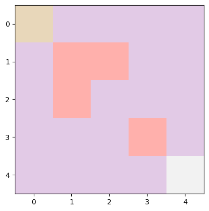
To make this more clear, imagine a simple 5×5 grid. Here, states are where the agent is on the grid, marked by coordinates (x,y), with x being the row and y the column. In a 5×5 grid, there are 25 possible spots, from the top-left corner (0,0) to the bottom-right (4,4), covering everything in between.
Let’s say the agent’s mission is to navigate from a starting point to a goal, dodging obstacles along the way. Picture this grid: the start is a yellow block at the top-left, the goal is a light grey block at the bottom-right, and there are pink blocks as obstacles.
Grid Environment — Image by Author
In a bit of code to set up this scenario, we’d define the grid’s size (5×5), the start point (0,0), the goal (4,4), and any obstacles. The agent’s current state starts at the beginning point, and we sprinkle in some obstacles for an extra challenge.
class GridWorld:
    def __init__(self, width: int = 5, height: int = 5, start: tuple = (0, 0), goal: tuple = (4, 4), obstacles: list = None):
        self.width = width
        self.height = height
        self.start = np.array(start)
        self.goal = np.array(goal)
        self.obstacles = [np.array(obstacle) for obstacle in obstacles] if obstacles else []
        self.state = self.start
Here’s a peek at what that setup might look like in code. We set the grid to be 5×5, with the starting point at (0,0) and the goal at (4,4). We keep track of the agent’s current spot with self.state, starting at the start point. And we add obstacles to mix things up.
If this snippet of code seems a bit much right now, no worries! We’ll dive into a detailed example later on, making everything crystal clear.
Actions
Actions are the choices available to the agent that can change the state.
Actions are what an agent can do to change its current state. If we stick with the video game example, actions might include moving left or right, jumping, or doing something specific like shooting. The collection of all actions an agent can take at any point is known as the action space. This space can be discrete, meaning there’s a set number of actions, or continuous, where actions can vary within a range.
In math terms, we express an action as a ∈ A(s), where A represents the action space, and A(s) is the set of all possible actions in state s. Actions can be either discrete or continuous, just like states.
Going back to our simpler grid example, let’s define our possible moves:
Each action is represented by a tuple showing the change in position. So, to move down from the starting point (0,0) to (1,0), you’d adjust one row down. To move right, you go from (1,0) to (1,1) by changing one column. To transition from one state to the next, we simply add the action’s effect to the current position.
However, our grid world has boundaries and obstacles to consider, so we’ve got to make sure our moves don’t lead us out of bounds or into trouble. Here’s how we handle that:
# Check for boundaries and obstacles
if 0 <= next_state[0] < self.height and 0 <= next_state[1] < self.width and next_state not in self.obstacles:
    self.state = next_state
This piece of code checks if the next move keeps us within the grid and avoids obstacles. If it does, the agent can proceed to that next spot.
So, actions are all about making moves and navigating the environment, considering what’s possible and what’s off-limits due to the layout and rules of our grid world.
Rewards
Rewards are immediate feedback received from the environment following an action.
Rewards are like instant feedback that the agent gets from the environment after it makes a move. Think of them as points that show whether an action was beneficial or not. The agent’s main aim is to collect as many points as possible over time, which means it has to think about both the short-term gains and the long-term impacts of its actions. Just like we mentioned earlier with the dog training analogy when a dog does something good, we give it a treat; if not, there might be a mild telling-off. This idea is pretty much a staple in reinforcement learning.
Mathematically, we describe a reward that comes from making a move a in state s and moving to a new state s′ as R(s, a, s′). Rewards can be either positive (like a treat) or negative (more like a gentle scold), and they’re crucial for helping the agent learn the best actions to take.
In our grid world scenario, we want to give the agent a big thumbs up if it reaches its goal. And because we value efficiency, we’ll deduct points for every move it makes that doesn’t succeed. In code, we’d set up a reward system somewhat like this:
reward = 100 if (self.state == self.goal).all() else -1
This means the agent gets a whopping 100 points for landing on the goal but loses a point for every step that doesn’t get it there. It’s a simple way to encourage our agent to find the quickest route to its target.
The Concept of Episodes and Policy
Understanding episodes and policy is key to getting how agents learn and decide what to do in reinforcement learning (RL) environments. Let’s dive into these concepts:
Episodes
An episode in reinforcement learning is a sequence of steps that starts in an initial state and ends when a terminal state is reached.
Think of an episode in reinforcement learning as a complete run of activity, starting from an initial point and ending when a specific goal is reached or a stopping condition is met. During an episode, the agent goes through a series of steps: it checks out the current situation (state), makes a move (action) based on its strategy (policy), and then gets feedback (reward) and the new situation (next state) from the environment. Episodes neatly package the agent’s experiences in scenarios where tasks have a clear start and finish.
In a video game, an episode might be tackling a single level, kicking off at the start of the level and wrapping up when the player either wins or runs out of lives.
In financial trading, an episode could be framed as a single trading day, starting when the market opens and ending at the close.
Episodes are useful because they let us measure how well different strategies (policies) work over a set period and help in learn from a full experience. This setup gives the agent chances to restart, apply what it’s learned, and experiment with new tactics under similar conditions.
Mathematically, you can visualize an episode as a series of moments:
Series of Moments — Image by Author
where:
st is the state at the time t
at is the action taken at the time t
rt+1 is the reward received after the action at
T marks the end of the episode
This sequence helps in tracking the flow of actions, states, and rewards throughout an episode, providing a framework for learning and improving strategies.
Policy
A policy is the strategy that an RL agent employs to decide which actions to take in various states.
In the world of reinforcement learning (RL), a policy is essentially the game plan an agent follows to decide its moves in different situations. It’s like a guidebook that maps out which actions to take when faced with various scenarios. Policies can come in two flavors: deterministic and stochastic.
Deterministic Policy A deterministic policy is straightforward: for any specific situation, it tells the agent exactly what to do. If you find yourself in a state s, the policy has a predefined action a ready to go. This kind of policy always picks the same action for a given state, making it predictable. You can think of a deterministic policy as a direct function that links states to their corresponding actions:
Deterministic Policy Formula — Image by Author
where a is the action chosen when the agent is in state s.
Stochastic Policy On the flip side, a stochastic policy adds a bit of unpredictability to the mix. Instead of a single action, it gives a set of probabilities for choosing among available actions in a given state. This randomness is crucial for exploring the environment, especially when the agent is still figuring out which actions work best. A stochastic policy is often expressed as a probability distribution over actions given a state s, symbolized as π(a ∣ s), indicating the likelihood of choosing action a when in state s:
Stochastic Policy Formula — Image by Author
where P denotes the probability.
The endgame of reinforcement learning is to uncover the optimal policy, one that maximizes the total expected rewards over time. Finding this balance between exploring new actions and exploiting known lucrative ones is key. The idea of an “optimal policy” ties closely to the value function concept, which gauges the anticipated rewards (or returns) from each state or action-state pairing, based on the policy in play. This journey of exploration and exploitation helps the agent learn the best paths to take, aiming for the highest cumulative reward.
Mathematical Formulation of the RL Problem
The way reinforcement learning (RL) problems are set up mathematically is key to understanding how agents learn to make smart decisions that maximize their rewards over time. This setup involves a few main ideas: the objective function, return (or cumulative reward), discounting, and the overall goal of optimization. Let’s dig into these concepts:
Objective Function
At the core of RL is the objective function, which is the target that the agent is trying to hit by interacting with the environment. Simply put, the agent wants to collect as many rewards as it can. We measure this goal using the expected return, which is the total of all rewards the agent thinks it can get, starting from a certain point and following a specific game plan or policy.
Return (Cumulative Reward)
“Return” is the term used for the total rewards that an agent picks up, whether that’s in one go (a single episode) or over a longer period. You can think of it as the agent’s score, where every move it makes either earns or loses points based on how well it turns out. If we’re not thinking about discounting for a moment, the return is just the sum of all rewards from each step t until the episode ends:
Return Formula — Image by Author
Here, Rt represents the reward obtained at time t, and T marks the episode’s conclusion.
Discounting
In RL, not every reward is seen as equally valuable. There’s a preference for rewards received sooner rather than later, and this is where discounting comes into play. Discounting reduces the value of future rewards with a discount factor γ, which is a number between 0 and 1. The discounted return formula looks like this:
Discounting Formula — Image by Author
This approach keeps the agent’s score from blowing up to infinity, especially when we’re looking at endless scenarios. It also encourages the agent to prioritize actions that deliver rewards more quickly, balancing the pursuit of immediate versus future gains.
Building an RL Environment
Now, let’s take the grid example we talked about earlier, and write a code to implement an agent navigating through the environment and reaching its goal. Let’s construct a straightforward grid world environment, outline a navigation policy for our agent, and kick off a simulation to see everything in action.
Let’s first show all the code and then let’s break it down.
import numpy as np import matplotlib.pyplot as plt import logging logging.basicConfig(level=logging.INFO)
class GridWorld: """ GridWorld environment for navigation.
Args: - width: Width of the grid - height: Height of the grid - start: Start position of the agent - goal: Goal position of the agent - obstacles: List of obstacles in the grid
Methods: - reset: Reset the environment to the start state - is_valid_state: Check if the given state is valid - step: Take a step in the environment """ def __init__(self, width: int = 5, height: int = 5, start: tuple = (0, 0), goal: tuple = (4, 4), obstacles: list = None): self.width = width self.height = height self.start = np.array(start) self.goal = np.array(goal) self.obstacles = [np.array(obstacle) for obstacle in obstacles] if obstacles else [] self.state = self.start self.actions = {'up': np.array([-1, 0]), 'down': np.array([1, 0]), 'left': np.array([0, -1]), 'right': np.array([0, 1])}
def reset(self): """ Reset the environment to the start state
Returns: - Start state of the environment """ self.state = self.start return self.state
def is_valid_state(self, state): """ Check if the given state is valid
Args: - state: State to be checked
Returns: - True if the state is valid, False otherwise """ return 0 <= state[0] < self.height and 0 <= state[1] < self.width and all((state != obstacle).any() for obstacle in self.obstacles)
def step(self, action: str): """ Take a step in the environment
def navigation_policy(state: np.array, goal: np.array, obstacles: list): """ Policy for navigating the agent in the grid world environment
Args: - state: Current state of the agent - goal: Goal state of the agent - obstacles: List of obstacles in the environment
Returns: - Action to be taken by the agent """ actions = ['up', 'down', 'left', 'right'] valid_actions = {} for action in actions: next_state = state + env.actions[action] if env.is_valid_state(next_state): valid_actions[action] = np.sum(np.abs(next_state - goal)) return min(valid_actions, key=valid_actions.get) if valid_actions else None
def run_simulation_with_policy(env: GridWorld, policy): """ Run the simulation with the given policy
Args: - env: GridWorld environment - policy: Policy to be used for navigation """ state = env.reset() done = False logging.info(f"Start State: {state}, Goal: {env.goal}, Obstacles: {env.obstacles}") while not done: # Visualization grid = np.zeros((env.height, env.width)) grid[tuple(state)] = 1 # current state grid[tuple(env.goal)] = 2 # goal for obstacle in env.obstacles: grid[tuple(obstacle)] = -1 # obstacles
plt.imshow(grid, cmap='Pastel1') plt.show()
action = policy(state, env.goal, env.obstacles) if action is None: logging.info("No valid actions available, agent is stuck.") break next_state, reward, done = env.step(action) logging.info(f"State: {state} -> Action: {action} -> Next State: {next_state}, Reward: {reward}") state = next_state if done: logging.info("Goal reached!")
# Define obstacles in the environment obstacles = [(1, 1), (1, 2), (2, 1), (3, 3)]
# Create the environment with obstacles env = GridWorld(obstacles=obstacles)
# Run the simulation run_simulation_with_policy(env, navigation_policy)
class GridWorld:
    def __init__(self, width: int = 5, height: int = 5, start: tuple = (0, 0), goal: tuple = (4, 4), obstacles: list = None):
        self.width = width
        self.height = height
        self.start = np.array(start)
        self.goal = np.array(goal)
        self.obstacles = [np.array(obstacle) for obstacle in obstacles] if obstacles else []
        self.state = self.start
        self.actions = {'up': np.array([-1, 0]), 'down': np.array([1, 0]), 'left': np.array([0, -1]), 'right': np.array([0, 1])}
This class initializes a grid environment with a specified width and height, a start position for the agent, a goal position to reach, and a list of obstacles. Note that obstacles are a list of tuples, where each tuple represents the position of each obstacle.
Here, self.actions defines possible movements (up, down, left, right) as vectors that will modify the agent’s position.
reset() method sets the agent’s state back to the start position. This is useful when we want to train the agent several times, after each completion of the reach of a certain status, the agent will start back from the beginning.
def is_valid_state(self, state):
    return 0 <= state[0] < self.height and 0 <= state[1] < self.width and all((state != obstacle).any() for obstacle in self.obstacles)
is_valid_state(state) checks if a given state is within the grid boundaries and not an obstacle.
step(action: str) moves the agent according to the action if it’s valid, updates the state, calculates the reward, and checks if the goal is reached.
Navigation Policy Function
def navigation_policy(state: np.array, goal: np.array, obstacles: list):
    actions = ['up', 'down', 'left', 'right']
    valid_actions = {}
    for action in actions:
        next_state = state + env.actions[action]
        if env.is_valid_state(next_state):
            valid_actions[action] = np.sum(np.abs(next_state - goal))
    return min(valid_actions, key=valid_actions.get) if valid_actions else None
Defines a simple policy to decide the next action based on minimizing the distance to the goal while considering valid actions only. Indeed, for every valid action we calculate the distance between the new state and the goal, then we select the action that minimizes the distance. Keep in mind, that the function to calculate the distance is crucial for a performant RL agent. In this case, we are using a Manhattan distance calculation, but this may not be the best choice for different and more complex scenarios.
Simulation Function
def run_simulation_with_policy(env: GridWorld, policy):
    state = env.reset()
    done = False
    logging.info(f"Start State: {state}, Goal: {env.goal}, Obstacles: {env.obstacles}")
    while not done:
        # Visualization
        grid = np.zeros((env.height, env.width))
        grid[tuple(state)] = 1  # current state
        grid[tuple(env.goal)] = 2  # goal
        for obstacle in env.obstacles:
            grid[tuple(obstacle)] = -1  # obstacles

        plt.imshow(grid, cmap='Pastel1')
        plt.show()

        action = policy(state, env.goal, env.obstacles)
        if action is None:
            logging.info("No valid actions available, agent is stuck.")
            break
        next_state, reward, done = env.step(action)
        logging.info(f"State: {state} -> Action: {action} -> Next State: {next_state}, Reward: {reward}")
        state = next_state
        if done:
            logging.info("Goal reached!")
run_simulation_with_policy(env: GridWorld, policy) resets the environment and iteratively applies the navigation policy to move the agent towards the goal. It visualizes the grid and the agent’s progress at each step.
The simulation runs until the goal is reached or no valid actions are available (the agent is stuck).
Running the Simulation
# Define obstacles in the environment
obstacles = [(1, 1), (1, 2), (2, 1), (3, 3)]

# Create the environment with obstacles
env = GridWorld(obstacles=obstacles)

# Run the simulation
run_simulation_with_policy(env, navigation_policy)
The simulation is run using run_simulation_with_policy, applying the defined navigation policy to guide the agent.
Agent moving towards a goal — GIF by Author
By developing this RL environment and simulation, you get a firsthand look at the basics of agent navigation and decision-making, foundational concepts in the field of reinforcement learning.
Next Steps
As we delve deeper into the world of reinforcement learning (RL), it’s important to take stock of where we currently stand. Here’s a rundown of what our current approach lacks and our plans for bridging these gaps:
Current Shortcomings
Static Environment Our simulations run in a fixed grid world, with unchanging obstacles and goals. This setup doesn’t challenge the agent with new or evolving obstacles, limiting its need to adapt or strategize beyond the basics.
Basic Navigation Policy The policy we’ve implemented is quite basic, focusing solely on obstacle avoidance and goal achievement. It lacks the depth required for more complex decision-making or learning from past interactions with the environment.
No Learning Mechanism As it stands, our agent doesn’t learn from its experiences. It reacts to immediate rewards without improving its approach based on past actions, missing out on the essence of RL: learning and improving over time.
Absence of MDP Framework Our current model does not explicitly utilize the Markov Decision Process (MDP) framework. MDPs are crucial for understanding the dynamics of state transitions, actions, and rewards, and are foundational for advanced learning algorithms like Q-learning.
Expanding Horizons: The Road Ahead
Recognizing these limitations is the first step toward enhancing our RL exploration. Here’s what we plan to tackle in the next article:
Dynamic Environment We’ll upgrade our grid world to introduce elements that change over time, such as moving obstacles or changing rewards. This will compel the agent to continuously adapt its strategies, offering a richer, more complex learning experience.
Implementing Q-learning To give our agent the ability to learn and evolve, we’ll introduce Q-learning. This algorithm is a game-changer, enabling the agent to accumulate knowledge and refine its strategies based on the outcomes of past actions.
Exploring MDPs Diving into the Markov Decision Process will provide a solid theoretical foundation for our simulations. Understanding MDPs is key to grasping decision-making in uncertain environments, evaluating and improving policies, and how algorithms like Q-learning fit into this framework.
Complex Algorithms and Strategies With the groundwork laid by Q-learning and MDPs, we’ll explore more sophisticated algorithms and strategies. This advancement will not only elevate our agent’s intelligence but also its proficiency in navigating the intricacies of a dynamic and challenging grid world.
By addressing these areas, we aim to unlock new levels of complexity and learning in our reinforcement learning journey. The next steps promise to transform our simple agent into one capable of making informed decisions, adapting to changing environments, and continuously learning from its experiences.
Conclusion
Wrapping up our initial dive into the core concepts of reinforcement learning (RL) within the confines of a simple grid world, it’s clear we’ve only scratched the surface of what’s possible. This first article has set the stage, showcasing both the promise and the current constraints of our approach. The simplicity of our static setup and the basic nature of our navigation tactics have spotlighted key areas ready for advancement.
You made it to the end. Congrats! I hope you enjoyed this article. If so consider leaving a clap and following me, as I will regularly post similar articles. As with every beginning of a new series, this article may not be perfect, and with your input, it can highly improve. So, let me know what you think about it, what you would like to see more, and what less.
In 1965, cryogenics pioneer Olli V. Lounasmaa set up the Low Temperature Laboratory (LTL) at what is now Aalto University to research ultra-low temperature physics. Despite some initial scepticism because “why would anyone want to research cold in Finland,” the LTL has prospered, attracting researchers from all over the world — and laying the foundation for Finland’s leading quantum computing startup ecosystem. Quantum computing has long been the stuff of dreams. Arthur C. Clarke’s statement from the 1970s that “any sufficiently advanced technology is indistinguishable from magic,” has never felt truer than when trying to wrap one’s head around phenomena…
On this episode of HomeKit Insider, your hosts break down the latest rumors surrounding Apple’s rumored smart home display, look at some new trackers, and go hands-on with a Find My-enabled wallet.
HomeKit Insider Podcast
Once more, the recent beta of tvOS 17.4 has revealed more information regarding Apple’s purported smart home display. At this stage, a release may be sooner rather than later.
The device, known as Z314 internally, is running an A15 Bionic processor. The tvOS 17.4 beta included SwiftUI frameworks and a speific API, which would only be necessary for a device with a display.
Amazon’s under-the-radar discount on the M2 Pro Mac mini shaves $150 off the high-end model, matching the lowest price we’ve seen in 2024. Plus, snap up savings on every other configuration with prices as low as $499.
Save on Apple’s Mac mini at Amazon.
Amazon’s $1,149.99 price is in the form of a $100 instant rebate stacked with a $49.01 on-page coupon. This M2 Pro model (Apple’s latest Mac mini) is equipped with a 10-core CPU and 16-core GPU. It also has 16GB of memory and 512GB of storage, making it a popular choice among users looking to maintain a fixed office setup complete with an external monitor and peripherals.
Deals: Apple’s M2 Pro Mac mini drops to $1,149, best price of 2024
Originally appeared here:
Deals: Apple’s M2 Pro Mac mini drops to $1,149, best price of 2024
We use cookies on our website to give you the most relevant experience by remembering your preferences and repeat visits. By clicking “Accept”, you consent to the use of ALL the cookies.
This website uses cookies to improve your experience while you navigate through the website. Out of these, the cookies that are categorized as necessary are stored on your browser as they are essential for the working of basic functionalities of the website. We also use third-party cookies that help us analyze and understand how you use this website. These cookies will be stored in your browser only with your consent. You also have the option to opt-out of these cookies. But opting out of some of these cookies may affect your browsing experience.
Necessary cookies are absolutely essential for the website to function properly. These cookies ensure basic functionalities and security features of the website, anonymously.
Cookie
Duration
Description
cookielawinfo-checkbox-analytics
11 months
This cookie is set by GDPR Cookie Consent plugin. The cookie is used to store the user consent for the cookies in the category "Analytics".
cookielawinfo-checkbox-functional
11 months
The cookie is set by GDPR cookie consent to record the user consent for the cookies in the category "Functional".
cookielawinfo-checkbox-necessary
11 months
This cookie is set by GDPR Cookie Consent plugin. The cookies is used to store the user consent for the cookies in the category "Necessary".
cookielawinfo-checkbox-others
11 months
This cookie is set by GDPR Cookie Consent plugin. The cookie is used to store the user consent for the cookies in the category "Other.
cookielawinfo-checkbox-performance
11 months
This cookie is set by GDPR Cookie Consent plugin. The cookie is used to store the user consent for the cookies in the category "Performance".
viewed_cookie_policy
11 months
The cookie is set by the GDPR Cookie Consent plugin and is used to store whether or not user has consented to the use of cookies. It does not store any personal data.
Functional cookies help to perform certain functionalities like sharing the content of the website on social media platforms, collect feedbacks, and other third-party features.
Performance cookies are used to understand and analyze the key performance indexes of the website which helps in delivering a better user experience for the visitors.
Analytical cookies are used to understand how visitors interact with the website. These cookies help provide information on metrics the number of visitors, bounce rate, traffic source, etc.
Advertisement cookies are used to provide visitors with relevant ads and marketing campaigns. These cookies track visitors across websites and collect information to provide customized ads.