Essential Metrics and Methods to Enhance Performance Across Retrieval, Generation, and End-to-End Pipelines
Originally appeared here:
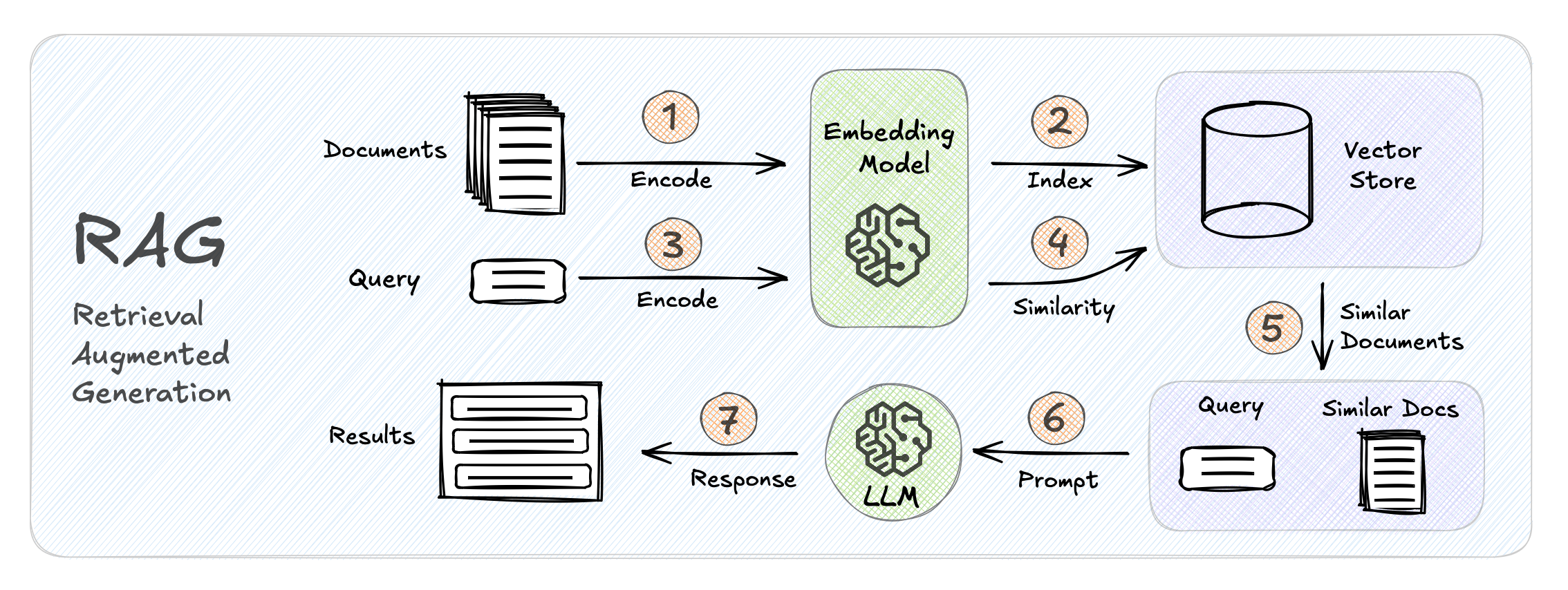
Unlocking the Untapped Potential of Retrieval-Augmented Generation (RAG) Pipelines
Essential Metrics and Methods to Enhance Performance Across Retrieval, Generation, and End-to-End Pipelines
Originally appeared here:
Unlocking the Untapped Potential of Retrieval-Augmented Generation (RAG) Pipelines
Tips on how to get started, write your first article, and get noticed
Originally appeared here:
How To Start A Data Science Blog on Medium
Go Here to Read this Fast! How To Start A Data Science Blog on Medium
In this 2021 post, I demonstrated how linear optimization problems could be solved using the Pyomo package in Python and the JuMP package in Julia. I also introduced different types of commercial and non-commercial solvers available for solving linear, mixed integer, or non-linear optimization problems.
In this post, I will introduce mathematical programming system (mps) files used to represent optimization problems, the optimization process of a solver, and the solution file formats. For this purpose, I will use the same problem as in the previous post but with additional bounds. I am going to use an open-source solver called HiGHS for this purpose. HiGHS has been touted as one of the most powerful solvers among the open-source ones to solve linear optimization problems. In Python, I get access to this solver simply by installing the highpy package with pip install highspy.
Without further ado, let’s get started.

The problem statement is given below. x and y are the two decision variables. The objective is to maximize profit subject to three constraints. Both x and y have lower and upper bounds respectively.
Profit = 90x + 75y
Objective: maximize Profit subject to:
3x+2y≤66
9x+4y≤180
2x+10y≤200

Bounds:
2≤x≤8
10≤y≤40
In the code below, I initiate the model as h. Then, I introduce my decision variables x and y along with their lower bounds and upper bounds respectively, and also assign the names. Next, I add the three constraint inequalities which I have referred to as c0, c1 and c2 respectively. Each constraint has coefficient for x and y, and a RHS value. Then, I maximized the value of 90x+75y, which is the objective function. The model is run in this line.
import highspy
import numpy as np

#initiate the model
h = highspy.Highs()

#define decision variables
x = h.addVariable(lb = 2, ub = 8, name = “x”)
y = h.addVariable(lb = 10, ub = 40, name = “y”)

#h.setOptionValue("solver", "ipm")

#define constraints
h.addConstr(3*x + 2*y<=66) #c0
h.addConstr(9*x + 4*y<=180) #c1
h.addConstr(2*x + 10*y<=200) #c2

#objective
h.maximize(90*x + 75*y)
When the model runs, one can see the following progress happening in the terminal window. But what exactly is going on here? I describe it below:
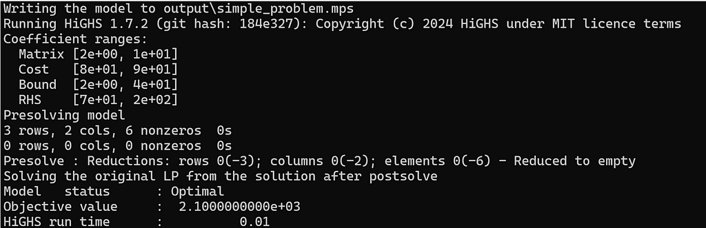
Problem size:
The constraints in the linear problem can be represented in the matrix form as Ax≤b, wherein, A is the matrix of constraint coefficients, x is the vector containing decision variables, and b is the matrix of RHS values. For the given problem, the constraints are represented in the matrix format as shown below:
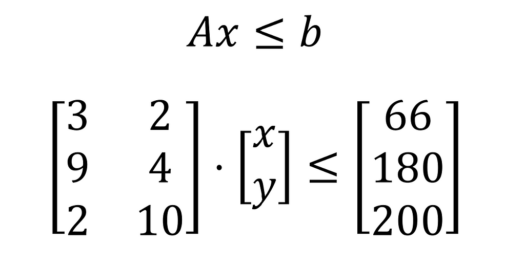
The problem matrix size is characterized by rows, columns and non-zero elements. Row refers to the number of constraints (here 3), column refers to the number of decision variables (here 2), and elements/non-zeros refer to the coefficients, which don’t have zero values. In all three constraints, there are no coefficient with zero value. Hence the total number of non-zero elements is six.
This is an example of a very simple problem. In reality, there can be problems where the number of rows, columns and non-zero elements can be in the order of thousands and millions. An increase in the problem size increases the complexity of the model, and the time taken to solve it.
Coefficient ranges
The coefficients of x and y in the problem range from 2 to 10. Hence, the matrix coefficient range is displayed as [2e+00, 1e+01].
Cost refers to the objective function here. Its coefficient is 90 for x and 75 for y. As a result, Cost has a coefficient range of [8e+01, 9e+01].
Bounds for x and y range between 2 and 40. Hence, Bound has a coefficient range of [2e+00, 4e+01]
Coefficients of RHS range between 66 and 200. Hence, RHS has a coefficient range of [7e+01, 2e+02].
Presolving
Presolve is the initial process when a solver tries to solve an optimization problem, it tries to simplify the model at first. For example, it might treat a coefficient beyond a certain value as infinity. The purpose of the presolve is to create a smaller version of the problem matrix, with identical objective function and with a feasible space that can be mapped to the feasible space of the original problem. The reduced problem matrix would be simpler, easier, and faster to solve than the original one.
In this case, the presolve step was completed in just two iterations resulting in an empty matrix. This also means that the solution was obtained and no further optimization was required. The objective value it returned was 2100, and the run time of the HiGHS solver was just 0.01 seconds. After the solution is obtained from the optimization, the solver can use the postsolve/unpresolve step wherein, the solution is mapped to the feasible space of the original problem.
Mathematical Programming System (MPS) is a file format for representing linear and mixed integer linear programming problems. It is a relatively old format but accepted by all commercial linear program solvers. Linear problems can also be written in other formats such as LP, AMPL, and GAMS.
One can use highspy to write mps file by simply using h.writeModel(“foo.mps”). And reading the mps file is as simple as h.readModel(“foo.mps”).
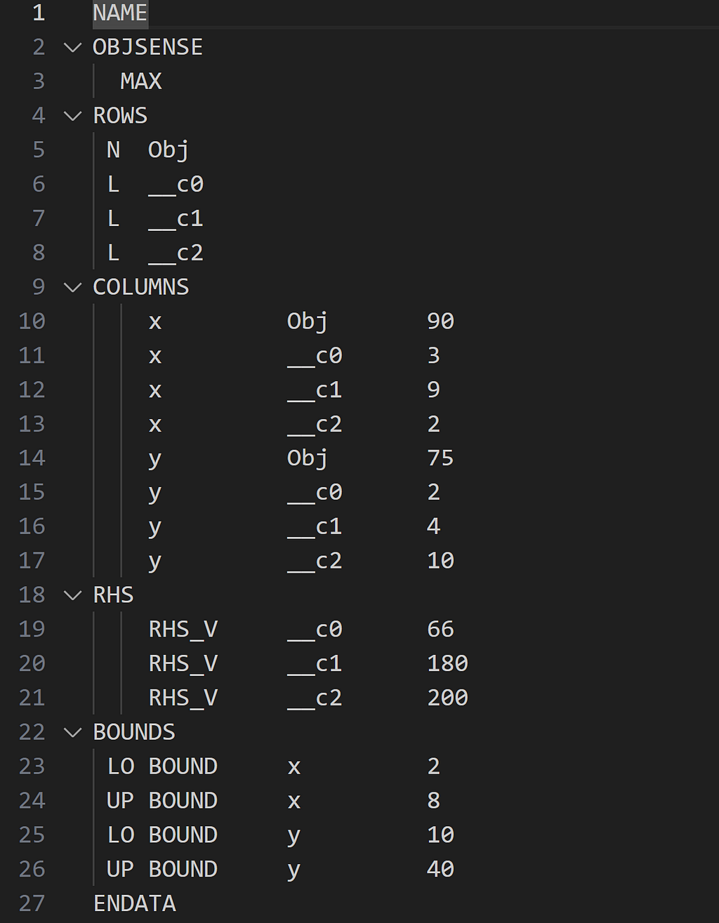
The structure of the MPS file of the given optimization problem is shown above. It starts with the NAME of the LP problem. OBJSENSE indicates whether the problem is a minimization (MIN) or maximization (MAX), here the latter. The ROWS section indicates the objective, names of all constraints, and their types in terms of equality/inequality. E stands for equality, G stands for greater than or equal rows, L stands for less than or equal rows, and N stands for no restriction rows. Here, the three constraints are given as __c0, __c1, and __c2 while Obj is the abbreviation for the objective.
In the COLUMNS section, the names of the decision variables (here x and y) are assigned on the left, and their coefficients which belong to objective or constraints inequalities are provided on the right. The RHS section contains the right-hand side vectors of the model constraints. The lower and upper bounds of the decision variables are defined in the BOUNDS section. The MPS file closes with ENDATA.
HiGHS uses algorithms such as simplex or interior point method for the optimization process. To explain these algorithms deserve a separate post of their own. I hope to touch upon them in the future.
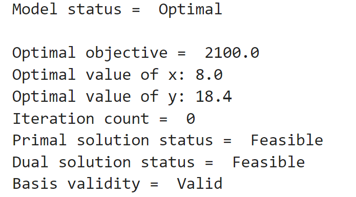
The code used to extract the results is given below. The model status is optimum. I extract the objective function value and the solution values of the decision variables. Furthermore, I print the number of iterations, the status of primal and dual solutions, and basis validity.
solution = h.getSolution()
basis = h.getBasis()
info = h.getInfo()

model_status = h.getModelStatus()
print("Model status = ", h.modelStatusToString(model_status))
print()

#Get solution objective value, and optimal values for x and y
print("Optimal objective = ", info.objective_function_value)
print ("Optimal value of x:", solution.col_value[0])
print ("Optimal value of y:", solution.col_value[1])

#get model run characteristics
print('Iteration count = ', info.simplex_iteration_count)
print('Primal solution status = ', h.solutionStatusToString(info.primal_solution_status))
print('Dual solution status = ', h.solutionStatusToString(info.dual_solution_status))
print('Basis validity = ', h.basisValidityToString(info.basis_validity))
After the optimization process, HiGHS allows writing the solution into a solution file with a .sol extension. Further, the solution can be written in different formats as given here. 1 stands for HiGHS pretty format, and 3 stands for Glpsol pretty format respectively.
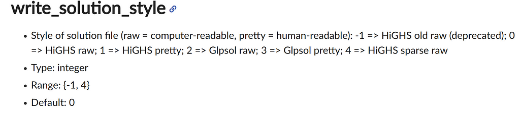
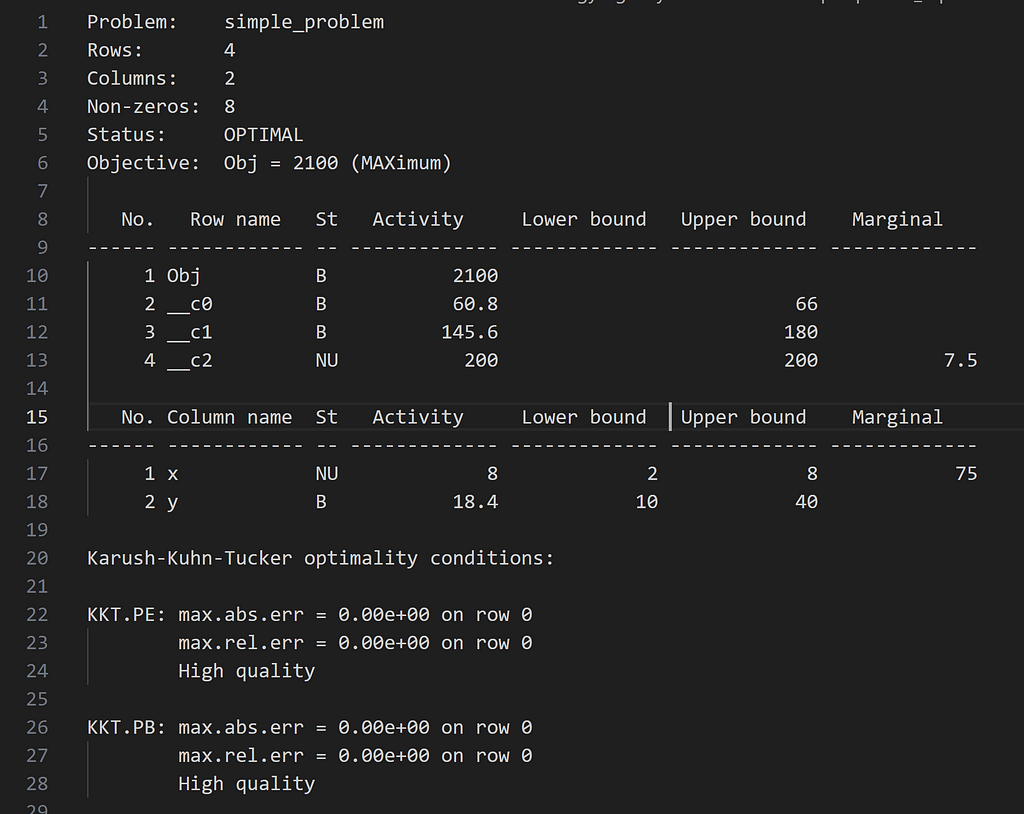
To get the solution in style 3, I used h.writeSolution(“mysolution.sol”, 3). The problem statistics are provided at the top. The optimal solution values are provided in the Activity column. The St column specifies the status of the solution. For example, B stands for Basic- the variable or constraint is part of the basis solution (optimal). NU refers that the solution is non-basic and is the same as the upper bound. The value in the Marginal column (often referred to as the shadow price or dual value) refers to how much the objective function would vary with the unit change in the non-basic variable. For more information on the GLPK solution file information, one can refer to here.
In this post, I presented an example of solving a simple linear optimization problem using an open-source solver called HiGHS with the highspy package in Python. Next, I explained how the optimization problem size can be inferred using the coefficient matrix, decision variable vector and RHS vector. I introduced and explained different components of mathematical programming system (mps) files for representing optimization problem. Finally, I demonstrated the optimization process of a solver, steps for extracting results and analyzing the solution file.
The notebook and relevant files for this post is available in this GitHub repository. Thank you for reading!
Understanding the Optimization Process Pipeline in Linear Programming was originally published in Towards Data Science on Medium, where people are continuing the conversation by highlighting and responding to this story.
Originally appeared here:
Understanding the Optimization Process Pipeline in Linear Programming
Go Here to Read this Fast! Understanding the Optimization Process Pipeline in Linear Programming
Go Here to Read this Fast! NASA’s exciting 2024 began with a crash that ended a historic mission
Originally appeared here:
NASA’s exciting 2024 began with a crash that ended a historic mission
The Steam Deck and ROG Ally are fun gaming machines, but we’ll always have a special place in our hearts for the Nintendo Switch and its fantastic game library that includes Zelda, Animal Crossing and, of course, Mario. You may be anticipating the launch of the next-gen console (we know we are), but that doesn’t mean you can’t enjoy the system you have in front of you right now. A great way to make that few-years-old Switch feel almost like new again is with a few choice accessories, and on top of that, they can make your gaming experience better both at home and on the go. We’ve chosen some of our favorite Switch accessories to give your system the royal treatment.
This article originally appeared on Engadget at https://www.engadget.com/gaming/nintendo/best-nintendo-switch-oled-accessories-150048703.html?src=rss
Go Here to Read this Fast! The best Nintendo Switch OLED accessories for 2025
Originally appeared here:
The best Nintendo Switch OLED accessories for 2025
Whether you’re playing on the original Nintendo Switch, the sleek handheld-only Switch Lite or the upgraded OLED model with its stunning display, you’re in for a gaming experience that’s versatile, immersive and downright fun. The beauty of the Switch lineup is that, despite having different models, all games are compatible across the board. So no matter which version you own, you’ll have access to the entire library of games without worrying about what works on which console. This flexibility makes the Switch lineup ideal for both casual gamers and hardcore fans who love having the ability to access every title, whether they’re at home on the big screen or gaming on the go.
With such a vast and diverse game library, choosing the best games can feel a bit overwhelming. Nintendo has something for everyone — from epic action adventures and thrilling multiplayer battles to relaxing life sims and nostalgic platformers that bring back memories of classic gaming days. Whether you’re looking to dive into sprawling RPGs, conquer puzzles or enjoy a bit of friendly competition, the Switch has you covered.
Check out our entire Best Games series including the best Nintendo Switch games, the best PS5 games, the best Xbox games, the best PC games and the best free games you can play today.
This article originally appeared on Engadget at https://www.engadget.com/gaming/nintendo/best-nintendo-switch-games-160029843.html?src=rss
Go Here to Read this Fast! The 26 best Nintendo Switch games in 2025
Originally appeared here:
The 26 best Nintendo Switch games in 2025


Originally appeared here:
I tried using smart home devices to help fix my irregular routine – and it changed my life

Originally appeared here:
NYT Wordle today — answer and my hints for game #1287, Friday, December 27


This story continues at The Next Web
Originally appeared here:
A rising tide of e-waste threatens our health, the environment and the economy