Razer brought a fancypants monitor stand to CES 2025 in Las Vegas, and this one features RGB lights. The Chroma stand is an ergonomic unit built from anodized aluminum, with a sleek black matte finish. It can support up to 44 pounds, which should easily accommodate most monitors.
The integrated RGB lighting supports up to 16.8 million colors and can run a series of lighting effects. Users create custom lighting profiles which can be cycled through via a remappable button. This button can also be used for other purposes, like launching applications or muting audio. Of course, it syncs up with other Chroma-capable devices to “create a cohesive, immersive aesthetic.” Yay, lighting!
Razer
Even if you hate custom lighting, there’s one thing we can all agree on. There are simply not enough ports in the world for all of our many gadgets. To that end, the Chroma Stand includes a built-in 4-port hub that connects via a single USB-C cable. The available ports include a pair of USB-A inputs, a single USB-C and an HDMI.
It doesn’t offer any adjustment capabilities, but the stand does include anti-slip rubber pads on the bottom for stability. There’s also an open space underneath, which is perfect for smartphones, laptops and other gadgets. The Razer Monitor Stand Chroma costs $200 and pre-orders are open right now.
This article originally appeared on Engadget at https://www.engadget.com/gaming/pc/razer-made-a-monitor-stand-with-rgb-lights-because-of-course-it-did-140029786.html?src=rss
Klipsch, a company more known for shelf speakers, towers and soundbars, is adding three more portable speakers to its Music City Party Speaker lineup. The original three speakers are the Austin, Nashville and Detroit models. At CES 2025, Klipsch is adding the Vegas, Miami and New York models.
The Vegas is the smallest model among the three and has a single 5.25-inch woofer, while the Miami is larger and has two 5.25-inch woofers for more bass. The New York is the biggest one and has dual eight-inch woofers. Other differences include the Vegas and Miami’s pole mounts for easy setup, which the New York doesn’t have. However, the New York and Miami have trolley wheels due to their larger size and heavier weight. These wheels make it easier to take the speakers on the road.
The new speakers all come with a karaoke microphone, handles for portability and some sound effects like audience cheering and an airhorn, along with RGB lighting for outdoor enjoyment. They also support Bluetooth 5.2 connections and have a Bass Boost mode if you think there isn’t enough low end. Additionally, if you have more than one of these speakers, Party Mode can link them up for a more immersive experience.
For sound customization, all three speakers work with the Klipsch Connect Plus app. The app supports EQ adjustments, RGB and light pattern changes and more. Klipsch says that the Vegas can last for eight hours of playing, while the Miami can reach 18 hours. The New York, despite being the largest of the trio, has a maximum battery life of 12 hours. Turning the lights on reduces battery life.
All three speakers will be available in Spring 2025. The Vegas will cost $299, the Miami goes for $549 and the New York can be yours for $699. You may pre-order them starting January 7, 2025.
This article originally appeared on Engadget at https://www.engadget.com/audio/speakers/klipsch-introduces-the-newest-music-city-party-karaoke-focused-speakers-140018483.html?src=rss
Netgear just announced a new Wi-Fi 7 mesh router system called the Orbi 870, joining the pre-existing 970 and 770. The company says that the latest system “offers the perfect balance of performance, coverage, and security.”
To that end, the Orbi 870 offers tri-band speeds up to 21Gbps and all kinds of modern bells and whistles. These include enhancements like support for the latest 320MHz bandwidth and 4K QAM, which squeezes more data into traditional transmissions. This looks to be a fairly future-proof router system.
Netgear also touts the reliability of this device, thanks to an enhanced backhaul that combines 5GHz and 6GHz into a single band. Of course, there are plenty of wired connectivity options here. There’s a 10 gigabit internet port and four 2.5Gbps Ethernet ports on the router. Additionally, each satellite includes four Ethernet ports.
Netgear
Like most Netgear mesh systems, adjustments can be made via the Orbi app. This lets users pause the internet, run speed tests, track usage and set up separate networks for guests. This app also allows access to parental controls.
The Netgear Orbi 870 system is available in black or white. A three-pack that includes the router and two satellites costs $1,300, while a two-pack costs $1,000. Additional satellites can be purchased for $550 each. This is expensive, to be sure, but an actual bargain when compared to the slightly higher-end Orbi 970 system.
This article originally appeared on Engadget at https://www.engadget.com/home/smart-home/netgears-orbi-870-mesh-router-system-is-a-great-way-to-join-the-wi-fi-7-bandwagon-133031270.html?src=rss
Bad actors have created deepfakes to imitate celebrity endorsements, President Biden and employers. But, one of the most heinous uses is making sexually explicit deepfakes of real people. Now, the UK government is taking new steps to deter their creation, introducing new criminal offenses for producing or sharing sexually explicit deepfakes. Only sharing deepfakes is currently an offense under UK law.
“With these new measures, we’re sending an unequivocal message: creating or sharing these vile images is not only unacceptable but criminal,” said Baroness Margaret Beryl Jones, minister for the future digital economy and online safety. “Tech companies need to step up too — platforms hosting this content will face tougher scrutiny and significant penalties.” The new offenses will be proposed in parliament under the Government’s Crime and Policing Bill.
A similar measure was proposed in April 2024 by the previous UK government under former Prime Minister Rishi Sunak. However, it only covered cases in which a person created the deepfake to “cause alarm, humiliation or distress to the victim,” creating a loophole for perpetrators to argue their case. The law never progressed as Sunak called a general election just one month later. Notably, the new measure covers only adults, as it is already illegal to create or share any sexually explicit images of children.
The UK government has also announced its intention to make it a criminal offense if a person takes intimate photos or video without consent. Additional offenses would look at whether it was created without consent and to cause alarm, distress, humiliation or sexual gratification for themselves or another. A person charged with one of these actions can face up to two years in custody.
The US has attempted to create helpful measures or individuals impacted by deepfakes. In 2024, the Senate passed the Disrupt Explicit Forged Images and Non-Consensual Edits Act (DEFIANCE Act), which would allow victims of sexually explicit deepfakes to sue the perpetrators. It would give the individual 10 years to sue for up to $150,000 or $250,000 if it relates to attempted sexual assault, stalking or harassment. However, it’s fate is unclear, having sat in limbo in the House of Representatives since last July.
This article originally appeared on Engadget at https://www.engadget.com/new-uk-law-would-criminalize-creating-sexually-explicit-deepfakes-132155132.html?src=rss
If there’s one certainty of 2025, it’s that there will be a plethora of new AI products. One of the first out of the gate comes from Philips Hue, which has announced AI-powered smart lighting for creating just the right mood for every setting.
Philips Hue is bringing an AI assistant to its Hue app that will create “personalized lighting scenes.” You can instruct the assistant through text or voice commands. For instance, you might say something like, “Create a scene for a dinner party” or write “Give me a scene for a quiet night in.” Philips Hue will also have a feedback feature so you can share if the ambience isn’t what you requested.
Philips Hue
As of now, there’s not an exact release date for the AI assistant, but Philips Hue states it will become available this year. It should be compatible with all of its lights. Other companies have created similar products, such as iConnectHue, which added AI-powered “magic scenes” in early 2023.
This article originally appeared on Engadget at https://www.engadget.com/ai/philips-hue-adds-ai-powered-lighting-options-to-its-app-131538165.html?src=rss
8Bitdo makes some of our favorite controllers for all manner of consoles and gaming rigs, and now you can pick an Xbox controller of theirs up for only $30. The 8Bitdo Ultimate Wired Controller for Xbox is 33 percent off and down to just about a record-low price. Considering first-party Xbox controllers can be around $60, this is an especially good deal.
This controller may be more affordable, but it’s not a cheap knockoff. It’s licensed by Xbox and compatible with the Xbox Series X, Series S, Xbox One and Windows 10 and above; that means you can switch back and forth and use it with your console and PC.
There are two extra buttons on the back that aren’t included with the official controller, which could be useful for mapping (particularly with PC games.) To that end, the controller offers custom button mapping and stick/trigger sensitivity for control over vibration.
The Hall effect joysticks and impulse triggers should increase both durability and sensitivity, while minimizing drift. There’s also a 3.5mm audio jack on the back to directly connect to headphones. Other features include a classic d-pad and an enhanced grip.
So what’s the catch? It’s right there in the name. This is a wired controller, which is both a blessing and a curse. Wired controllers offer reduced latency, making them the preferred choice for pro-level gamers, but keep folks tethered to a cable. It ships with a fairly long cable, at nearly ten feet, but the wireless range of a standard Bluetooth controller comes in at around 20 feet.
Follow @EngadgetDeals on Twitter and subscribe to the Engadget Deals newsletter for the latest tech deals and buying advice.
This article originally appeared on Engadget at https://www.engadget.com/deals/8bitdos-ultimate-wired-controller-for-xbox-drops-to-only-30-173842385.html?src=rss
In 2023, Shokz strayed from its bone conduction roots with a pair of “air conduction” open-ear wireless earbuds. While the Shokz OpenFit delivered better audio than bone conduction models, that wasn’t saying much. Their sound was still hit-or-miss, and some users had problems with their finicky touch controls. At CES 2025, the company is back with the $180 OpenFit 2, which apparently has solutions for both issues, as well as a new bone-conduction headset for office calls.
The Shokz OpenFit 2 has a woofer and tweeter in each earpiece for more dynamic sound. (The first-gen model only had a single driver for each ear.) The company also improved its bass algorithm, which “enhances dynamic low-frequency vibrations directly to your ear.”
Shokz
The open-ear buds’ design hasn’t changed dramatically from the original OpenFit: a hook still wraps around each ear with a bud resting just outside. But Shokz engineered the new model’s ear hook with a softer silicone (for greater comfort) and a tighter curve (for improved stability). The company says it “molds to the contours of your ear for a personalized, comfortable fit.” Each earpiece weighs 9.4g (0.33 oz). You can order it in black or beige.
The 2023 model used touch controls, which aren’t always the best input solution for earbuds’ small surfaces. So, the new model has physical multifunction buttons in addition to touch controls, which should help prevent or minimize accidental touches.
The OpenFit 2 is rated for up to 11 hours per charge (up from seven in the first-gen model) or 48 hours when factoring in the bundled charging case. They also have a better water resistance rating (IP55 vs. IP54 in the original) and Bluetooth 5.4.
Shokz
Shokz also has a new office headset, the OpenMeet, which seems like a redesigned spiritual successor to its OpenComm series. Like other workplace headsets, it looks a bit… goofy, with its long mic stem jutting out toward the mouth area. Similar to the OpenComm, the earpiece sits in front of the ear instead of on, in or around it. But a key difference is that OpenMeet’s band extends over the top of the head, not behind it.
The company says OpenMeet is designed to feel weightless, thanks to a five-point design that distributes its 78 g for minimal pressure. Its audio merges bone and air conduction, and the company says its (hilariously named) “LeakSlayer 3.0” tech helps minimize sound leakage to help keep your calls private.
OpenMeet uses a dual-mic system using Qualcomm’s cVc noise reduction, which Shokz claims reduces background noise by up to 98.6 percent. It has a dedicated mute button, Bluetooth 5.4 and up to 15 hours of battery life.
The Shokz OpenFit 2 is available today for $180 on the company website, Amazon and retail partners (including Best Buy and Target). Meanwhile, the OpenMeet headset is sold through the company’s business website.
This article originally appeared on Engadget at https://www.engadget.com/audio/headphones/the-shokz-openfit-2-promises-better-sound-and-longer-battery-life-130016786.html?src=rss
An overview of feature selection, and presentation of a rarely used but highly effective method (History-based Feature Selection), based on a regression model trained to estimate the predictive power of a given set of features
When working with prediction problems for tabular data, we often include feature selection as part of the process. This can be done for at least a few reasons, each important, but each quite different. First, it may done to increase the accuracy of the model; second, to reduce the computational costs of training and executing the model; and third, it may be done to make the model more robust and able to perform well on future data.
This article is part of a series looking at feature selection. In this and the next article, I’ll take a deep look at the first two of these goals: maximizing accuracy and minimizing computation. The following article will look specifically at robustness.
As well, this article introduces a feature selection method called History-based Feature Selection (HBFS). HBFS is based on experimenting with different subsets of features, learning the patterns as to which perform well (and which features perform well when included together), and from this, estimating and discovering other subsets of features that may work better still.
HBFS is described more thoroughly in the next article; this article provides some context, in terms of how HBFS compares to other feature selection methods. As well, the next article describes some experiments performed to evaluate HBFS, comparing it to other feature selection methods, which are described in this article.
As well as providing some background for the HBFS feature selection method, this article is useful for readers simply interested in feature selection generally, as it provides an overview of feature selection that I believe will be interesting to readers.
Feature selection for model accuracy
Looking first at the accuracy of the model, it is often the case that we find a higher accuracy (either cross validating, or testing on a separate validation set) by using fewer features than the full set of features available. This can be a bit unintuitive as, in principle, many models, including tree-based models (which are not always, but tend to be the best performing for prediction on tabular data), should ideally be able to ignore the irrelevant features and use only the truly-predictive features, but in practice, the irrelevant (or only marginally predictive) features can very often confuse the models.
With tree-based models, for example, as we go lower in the trees, the split points are determined based on fewer and fewer records, and selecting an irrelevant feature becomes increasingly possible. Removing these from the model, while usually not resulting in very large gains, often provides some significant increase in accuracy (using accuracy here in a general sense, relating to whatever metric is used to evaluate the model, and not necessarily the accuracy metric per se).
Feature selection to reduce computational costs
The second motivation for feature selection covered here is minimizing the computational costs of the model, which is also often quite important. Having a reduced number of features can decrease the time and processing necessary for tuning, training, evaluation, inference, and monitoring.
Feature selection is actually part of the tuning process, but here we are considering the other tuning steps, including model selection, selecting the pre-processing performed, and hyper-parameter tuning — these are often very time consuming, but less so with sufficient feature selection performed upfront.
When tuning a model (for example, tuning the hyper-parameters), it’s often necessary to train and evaluate a large number of models, which can be very time-consuming. But, this can be substantially faster if the number of features is reduced sufficiently.
These steps can be quite a bit slower if done using a large number of features. In fact, the costs of using additional features can be significant enough that they outweigh the performance gains from using more features (where there are such gains — as indicated, using more features will not necessarily increase accuracy, and can actually lower accuracy), and it may make sense to accept a small drop in performance in order to use fewer features.
Additionally, it may be desirable to reduce inference time. In real-time environments, for example, it may be necessary to make a large number of predictions very quickly, and using simpler models (including using fewer features) can facilitate this in some cases.
There’s a similar cost with evaluating, and again with monitoring each model (for example, when performing tests for data drift, this is simpler where there are fewer features to monitor).
The business benefits of any increase in accuracy would need to be balanced with the costs of a more complex model. It’s often the case that any gain in accuracy, even very small, may make it well worth adding additional features. But the opposite is often true as well, and small gains in performance do not always justify the use of larger and slower models. In fact, very often, there is no real business benefit to small gains in accuracy.
Additional motivations
There can be other motivations as well for feature selection. In some environments, using more features than are necessary requires additional effort in terms of collecting, storing, and ensuring the quality of these features.
Another motivation, at least when working in a hosted environments, is that it may be that using fewer features can result in lower overall costs. This may be due to costs even beyond the additional computational costs when using more features. For example, when using Google BigQuery, the costs of queries are tied to the number of columns accessed, and so there may be cost savings where fewer features are used.
Techniques for Feature Selection
There are many ways to perform feature selection, and a number of ways to categorize these. What I’ll present here isn’t a standard form of classification for feature selection methods, but I think is a quite straight-forward and useful way to look at this. We can think of techniques as falling into two groups:
Methods that evaluate the predictive power of each feature individually. These include what are often referred to as filter methods, as well as some more involved methods. In general, methods in this category evaluate each feature, one at at time, in some way — for example, with respect to their correlation with the target column, or their mutual information with the target, and so on. These methods do not consider feature interactions, and may miss features that are predictive, but only when used in combination with other features, and may include features that are predictive, but highly redundant — where there are one or more features that add little additional predictive power given the presence of other features.
Methods that attempt to identify an ideal set of features. This includes what are often called wrapper methods (I’ll describe these further below). This also includes genetic methods, and other such optimization methods (swarm intelligence, etc.). These methods do not attempt to rank the predictive power of each individual feature, only to find a set of features that, together, work better than any other set. These methods typically evaluate a number of candidate feature sets and then select the best of these. Where these methods differ from each other is largely how they determine which feature sets to evaluate.
We’ll look at each of these categories a little closer next.
Estimating the predictive power of each feature individually
There are a number of methods for feature selection provided by scikit-learn (as well as several other libraries, for example, mlxtend).
The majority of the feature selection tools in scikit-learn are designed to identify the most predictive features, considering them one at a time, by evaluating their associations with the target column. These include, for example, chi2, mutual information, and the ANOVA f-value.
The FeatureEngine library also provides an implementation of an algorithm called MRMR, which similarly seeks to rank features, in this case based both on their association with the target, and their association with the other features (it ranks features highest that have high association with the target, and low association with the other features).
We’ll take a look next at some other methods that attempt to evaluate each feature individually. This is far from a complete list, but covers many of the most popular methods.
Recursive Feature Elimination
Recursive Feature Elimination, provided by scikit-learn, works by training a model first on the full set of features. This must be a model that is able to provide feature importances (for example Random Forest, which provides a feature_importance_ attribute, or Linear Regression, which can use the coefficients to estimate the importance of each feature, assuming the features have been scaled).
It then repeatedly removes the least important features, and re-evaluates the features, until a target number of features is reached. Assuming this proceeds until only one feature remains, we have a ranked order of the predictive value of each feature (the later the feature was removed, the more predictive it is assumed to be).
1D models
1D models are models that use one dimension, which is to say, one feature. For example, we may create a decision tree trained to predict the target using only a single feature. It’s possible to train such a decision tree for each feature in the data set, one at a time, and evaluate each’s ability to predict the target. For any features that are predictive on their own, the associated decision tree will have better-than-random skill.
Using this method, it’s also possible to rank the features, based on the accuracies of the 1D models trained using each feature.
This is somewhat similar to simply checking the correlation between the feature and target, but is also able to detect more complex, non-monotonic relationships between the features and target.
Model-based feature selection
Scikit-learn provides support for model-based feature selection. For this, a model is trained using all features, as with Recursive Feature Elimination, but instead of removing features one at a time, we simply use the feature importances provided by the model (or can do something similar, using another feature importance tool, such as SHAP). For example, we can train a LogisticRegression or RandomForest model. Doing this, we can access the feature importances assigned to each feature and select only the most relevant.
This is not necessarily an effective means to identify the best subset of features if our goal is to create the most accurate model we can, as it identifies the features the model is using in any case, and not the features it should be using. So, using this method will not tend to lead to more accurate models. However, this method is very fast, and where the goal is not to increase accuracy, but to reduce computation, this can be very useful.
Permutation tests
Permutation tests are similar. There are variations on how this may be done, but to look at one approach: we train a model on the full set of features, then evaluate it using a validation set, or by cross-validation. This provides a baseline for how well the model performs. We can then take each feature in the validation set, one at a time, and scramble (permute) it, re-evaluate the model, and determine how much the score drops. It’s also possible to re-train with each feature permuted, one a time. The greater the drop in accuracy, the more important the feature.
The Boruta method
With the Boruta method, we take each feature, and create what’s called a shadow feature, which is a permuted version of the original feature. So, if we originally have, say, 10 features in a table, we create shadow versions of each of these, so have 20 features in total. We then train a model using the 20 features and evaluate the importance of each feature. Again, we can use built-in feature importance measures as are provided by many scikit-learn models and other models (eg CatBoost), or can use a library such as SHAP (which may be slower, but will provide more accurate feature importances).
We take the maximum importance given to any of the shadow features (which are assumed to have zero predictive power) as the threshold separating predictive from non-predictive features. All other features are checked to see if their feature importance was higher than this threshold or not. This process is repeated many times and each feature is scored based on the number of times it received a feature importance higher than this threshold.
That’s a quick overview of some of the methods that may be used to evaluate features individually. These methods can be sub-optimal, particularly when the goal is to create the most accurate model, as they do not consider feature interactions, but they are very fast, and to tend to rank the features well.
Generally, using these, we will get a ranked ordering of each feature. We may have determined ahead of time how many features we wish to use. For example, if we know we wish to use 10 features, we can simply take the top 10 ranked features.
Or, we can test with a validation set, using the top 1 feature, then the top 2, then top 3, and so on, up to using all features. For example, if we have a rank ordering (from strongest to weakest) of the features: {E, B, H, D, G, A, F, C}, then we can test: {E}, then {E, B}, then {E, B, H} and so on up to the full set {E, B, H, D, G, A, F, C}, with the idea that if we used just one feature, it would be the strongest one; if we used just two features, it would be the strongest two, and so on. Given the scores for each of these feature sets, we can take either the number of features with the highest metric score, or the number of features that best balances score and number of features.
Finding the optimum subset of features
The main limitation of the above methods is that they don’t fully consider feature interactions. In particular, they can miss features that would be useful, even if not strong on their own (they may be useful, for example, in some specific subsets of the data, or where their relationship with another feature is predictive of the target), and they can include features that are redundant. If two or more features provide much of the same signal, most likely some of these can be removed with little drop in the skill of the model.
We look now at methods that attempt to find the subset of features that works optimally. These methods don’t attempt to evaluate or rank each feature individually, only to find the set of features that work the best as a set.
In order to identify the optimal set of features, it’s necessary to test and evaluate many such sets, which is more expensive — there are more combinations than when simply considering each feature on its own, and each combination is more expensive to evaluate (due to having more features, the models tend to be slower to train). It does, though, generally result in stronger models than when simply using all features, or when relying on methods that evaluate the features individually.
I should note, though, it’s not necessarily the case that we use strictly one or the other method; it’s quite possible to combine these. For example, as most of the methods to identify an optimal set of features are quite slow, it’s possible to first run one of the above methods (that evaluate the features individually and then rank their predictive power) to create a short list of features, and then execute a method to find the optimal subset of these shortlisted features. This can erroneously exclude some features (the method used first to filter the features may remove some features that would be useful given the presence of some other features), but can also be a good balance between faster but less accurate, and slower but more accurate, methods.
Methods that attempt to find the best set of features include what are called wrapper methods, random search, and various optimization methods, as well as some other approaches. The method introduced in this article, HBFS, is also an example of a method that seeks to find the optimal set of features. These are described next.
Wrapper methods
Wrapper methods also can be considered a technique to rank the features (they can provide a rank ordering of estimated predictive power), but for this discussion, I’ll categorize them as methods to find the best set of features it’s able to identify. Wrapper methods do actually test full combinations of features, but in a restricted (though often still very slow) manner.
With wrapper methods, we generally start either with an empty set of features, and add features one at a time (this is referred to as an additive process), or start with the complete set of features, and remove features one at a time (this is referred to as a subtractive process).
With an additive process, we first find the single feature that allows us to create the strongest model (using a relevant metric). This requires testing each feature one at a time. We then find the feature that, when added to the set, allows us to create the strongest model that uses the first feature and a second feature. This requires testing with each feature other than the feature already present. We then select the third feature in the same way, and so on, up to the last feature, or until reaching some stopping condition (such as a maximum number of features).
If there are features {A, B, C, D, E, F, G, H, I, J} , there are 10 features. We first test all 10 of these one at a time (requiring 10 tests). We may find D works best, so we have the feature set {D}. We then test {D, A}, {D, B}, {D, C}, {D, E},…{D, J}, which is 9 tests, and take the strongest of these. We may find {D, E} works best, so have {D, E} as the feature set. We then test {D, E, A}, {D, E, B}, …{D, E, J}, which is 8 tests, and again take the strongest of these, and continue in this way. If the goal is to find the best set of, say, 5, features, we may end with, for example,{D, E, B, A, I}.
We can see how this may miss the best combination of 5 features, but will tend to work fairly well. In this example, this likely would be at least among the strongest subsets of size 5 that could be identified, though testing, as described in the next article, shows wrapper methods do tend to work less effectively than would be hoped.
And we can also see that it can be prohibitively slow if there are many features. With hundreds of features, this would be impossible. But, with a moderate number of features, this can work reasonably well.
Subtractive methods work similarly, but with removing a feature at each step.
Random Search
Random search is rarely used for feature selection, though is used in many other contexts, such as hyperparameter tuning. In the next article, we show that random search actually works better for feature selection than might be expected, but it does suffer from not being strategic like wrapper methods, and from not learning over time like optimization techniques or HBFS.
This can result in random searches unnecessarily testing candidates that are certain to be weak (for example, candidates feature sets that are very similar to other feature sets already tested, where the previously-tested sets performed poorly). It can also result in failing to test combinations of features that would reasonably appear to be the most promising given the other experiments performed so far.
Random search, though, is very simple, can be adequate in many situations, and often out-performs methods that evaluate the features individually.
Optimization techniques
There are a number of optimization techniques that may be used to identify an optimal feature set, including Hill Climbing, genetic methods Bayesian Optimization, and swarm intelligence, among others.
Here, we would start with a random set of features, then find a small modification (adding or removing a small number of features) that improves the set (testing several such small modifications and taking the best of these), and then find a small change that improves over that set of features, and so on, until some stopping condition is met (we can limit the time, the number of candidates considered, the time since the last improvement, or set some other such limit).
In this way, starting with a random (and likely poorly-performing) set of features, we can gradually, and repeatedly improve on this, discovering stronger and stronger sets of features until a very strong set is eventually discovered.
For example, we may randomly start with {B, F, G, H, J}, then find the small variation {B, C, F, G, H, J} (which adds feature C) works better, then that {B, C, F, H, J} (which removes feature G) works a bit better still, and so on.
In some cases, we may get stuck in local optima and another technique, called simulated annealing, may be useful to continue progressing. This allows us to occasionally select lower-performing options, which can help prevent getting stuck in a state where there is no small change that improves it.
Genetic algorithms work similarly, though at each step, many candidates are considered as opposed to just one, and combining is done as well as mutating (the small modifications done to a candidate set of features at each step in a hill climbing solution are similar to the modifications made to candidates in genetic algorithms, where they are known as mutations).
With combining, two or more candidates are selected and one or more new candidates is created based on some combination of these. For example, if we have two feature sets, it’s possible to take half the features used by one of these, along with half used by the other, remove any duplicated features, and treat this as a new candidate.
(In practice, the candidates in feature selection problems when using genetic methods would normally be formatted as a string of 0’s and 1’s — one value for each feature — in an ordered list of features, indicating if that feature is included in the set or not, so the process to combine two candidates would likely be slightly different than this example, but the same idea.)
With Bayesian Optimization, the idea to solving a problem such as finding an optimal set of features, is to first try a number of random candidates, evaluate these, then create a model that can estimate the skill of other sets of features based on what we learn from the candidates that have been evaluated so far.
For this, we use a type of regressor called a Gaussian Process, as it has the ability to not only provide an estimate for any other candidate (in this case, to estimate the metric score for a model that would be trained using this set of features), but to quantify the uncertainty.
For example, if we’ve already evaluated a given set of features, say, {F1, F2, F10, F23, F51} (and got a score of 0.853), then we can be relatively certain about the score predicted for a very similar feature set, say: {F1, F2, F10, F23, F51, F53}, with an estimated score of 0.858 — though we cannot be perfectly certain, as the one additional feature, F53, may provide a lot of additional signal. But our estimate would be more certain than with a completely different set of features, for example {F34, F36, F41, F62} (assuming nothing similar to this has been evaluated yet, this would have high uncertainty).
As another example, the set {F1, F2, F10, F23} has one fewer feature, F51. If F51 appears to be not predictive (given the scores given to other feature sets with and without F53), or appears to be highly redundant with, say, F1, then we can estimate the score for {F1, F2, F10, F23} with some confidence — it should be about the same as for {F1, F2, F10, F23, F51}. There is still significant uncertainty, but, again, much less that with a completely different set of features.
So, for any given set of features, the Gaussian Process can generate not only an estimate of the score it would receive, but the uncertainty, which is provided in the form of a credible interval. For example, if we are concerned with the macro f1 score, the Gaussian Process can learn to estimate the macro f1 score of any given set of features. For one set it may estimate, for example, 0.61, and it may also specify a credible interval of 0.45 to 0.77, meaning there’s a 90% (if we use 90% for the width of the credible interval) probability the f1 score would be between 0.45 and 0.77.
Bayesian Optimization works to balance exploration and exploitation. At the beginning of the process, we tend to focus more on exploring — in this case, figuring out which features are predictive, which features are best to include together and so on. Then, over time, we tend to focus more on exploiting — taking advantage of what we’ve learned to try to identify the most promising sets of features that haven’t been evaluated yet, which we then test.
Bayesian Optimization works by alternating between using what’s called an acquisition method to identify the next candidate(s) to evaluate, evaluating these, learning from this, calling the acquisition method again, and so on. Early on, the acquisition method will tend to select candidates that look promising, but have high uncertainty (as these are the ones we can learn the most from), and later on, the candidates that appear most promising and have relatively low uncertainty (as these are the ones most likely to outperform the candidates already evaluated, though tend to be small variations on the top-scored feature sets so far found).
In this article, we introduce a method called History-based Feature Selection (HBFS), which is probably most similar to Bayesian Optimization, though somewhat simpler. We look at this next, and in the next article look at some experiments comparing its performance to some of the other methods covered so far.
History-based Feature Selection
We’ve now gone over, admittedly very quickly, many of the other main options for feature selection commonly used today. I’ll now introduce History-based Feature Selection (HBFS). This is another feature selection method, which I’ve found quite useful, and which I’m not aware of another implementation of, or even discussion of, though the idea is fairly intuitive and straightforward.
Given there was no other implementation I’m aware of, I’ve created a python implementation, now available on github, HistoryBasedFeatureSelection.
This provides Python code, documentation, an example notebook, and a file used to test HBFS fairly thoroughly.
Even where you don’t actually use HBFS for your machine learning models, I hope you’ll find the approach interesting. The ideas should still be useful, and are a hopefully, at minimum, a good way to help think about feature selection.
I will, though, show that HBFS tends to work quite favourably compared to other options for feature selection, so it likely is worth looking at for projects, though the ideas are simple enough they can be coded directly — using the code available on the github page may be convenient, but is not necessary.
I refer to this method as History-based Feature Selection (HBFS), as it learns from a history of trying feature subsets, learning from their performance on a validation set, testing additional candidate sets of features, learning from these and so on. As the history of experiments progresses, the model is able to learn increasingly well which subsets of features are most likely to perform well.
The following is the main algorithm, presented as pseudo-code:
Loop a specfied number of times (by default, 20)
| Generate several random subsets of features, each covering about half
|     the features
| Train a model using this set of features using the training data
| Evaluate this model using the validation set
| Record this set of features and their evaluated score

Loop a specified number of times (by default, 10)
|   Train a RandomForest regressor to predict, for any give subset of
|      features, the score of a model using those features. This is trained
|      on the history of model evaluations of so far.
|
|   Loop for a specified number of times (by default, 1000)
|   |   Generate a random set of features
|   |   Use the RandomForest regressor estimate the score using this set
|   |     of features
|   |   Store this estimate
|
|   Loop over a specfied number of the top-estimated candidates from the
|   |       previous loop (by default, 20)
|   |   Train a model using this set of features using the training data
|   |   Evaluate this model using the validation set
|   |   Record this set of features and their evaluated score

output the full set of feature sets evaluated and their scores,
   sorted by scores
We can see, this is a bit simpler than with Bayesian Optimization, as the first iteration is completely focused on exploration (the candidates are generated randomly) and all subsequent iterations focus entirely on exploitation — there is not a gradual trend towards more exploitation.
This as some benefit, as the process normally requires only a small number of iterations, usually between about 4 and 12 or so (so there is less value in exploring candidate feature sets that appear to be likely weak). It also avoids tuning the process of balancing exploration and exploitation.
So the acquisition function is quite straightforward — we simply select the candidates that haven’t been tested yet but appear to be most promising. While this can (due to some reduction in exploration) miss some candidates with strong potential, in practice it appears to identify the strongest candidates reliably and quite quickly.
HBFS executes reasonably quickly. It’s of course slower then methods that evaluate each feature individually, but in terms of performance compares quite well to wrapper methods, genetic methods, and other methods that seek to find the strongest feature sets.
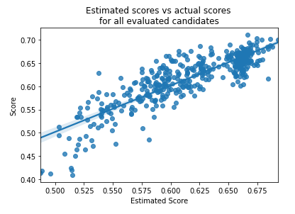
HBFS is designed to let users understand the feature-selection process it performs as it executes. For example, one of the visualizations provided plots the scores (both the estimated scores, and the actual-evaluated scores) for all feature sets that are evaluated, which helps us understand how well it’s able to estimate the the score that would be given for an arbitrary candidate feature set).
HBFS also includes some functionality not common with feature selection methods, such as allowing users to either: 1) simply maximize accuracy, or 2) to balance the goals of maximizing accuracy with minimizing computational costs. These are described in the next article.
Conclusions
This provided a quick overview of some of the most common methods for feature selection. Each works a bit differently and each has its pros and cons. Depending on the situation, and if the goal is to maximize accuracy, or to balance accuracy with computational costs, different methods can be preferable.
This also provided a very quick introduction to the History-based Feature Selection method.
HBFS is a new algorithm that I’ve found to work very well, and usually, though not always, preferably to the methods described here (no method will strictly out-perform all others).
In the next article we look closer at HBFS, as well as describe some experiments comparing its performance to some of the other methods described here.
In the following article, I’ll look at how feature selection can be used to create more robust models, given changes in the data or target that may occur in production.
Humor is an essential aspect of what makes humans, humans, but it is also an aspect that many contemporary AI models are very lacking in. They haven’t got a funny bone in them, not even a humerus. While creating and detecting jokes might seem unimportant, an LLM would likely be able to use this knowledge to craft even better, more human-like responses to questions. Understanding human humor also indicates a rudimentary understanding of human emotion and much greater functional competence.
Unfortunately, research into humor detection and classification still has several glaring issues. Most existing research either fails to apply existing linguistic and psychological theory to computation or fails to be interpretable enough to connect the model’s results and the theories of humor. That’s where the THInC (Theory-driven humor Interpretation and Classification) model comes in. This new approach, proposed by researchers from the University of Antwerp, the University of Leuven, and the University of Montreal at the 2024 European Conference on AI, seeks to leverage existing theories of humor through the use of Generalized Additive Models and pre-trained language transformers to create a highly accurate and interpretable humor detection methodology.
In this article, I aim to summarize the THInC framework and how Marez et al. approaches the difficult problem of humor detection. I recommend checking out their paper for more information.
Humor Theories
Before we dive into the computational approach of the paper, we need to first answer the question: what makes something funny? Well, one can look into humor Theories (insert citation here), various axioms that aim to explain why a joke could be considered a joke. There are countless humor theories, but there are three major ones that tend to take the spotlight:
Incongruity Theory: We find humor in events that are surprising or don’t fit our expectations of events playing out without being outright mortifying. It could just be a small deviation of the norm or a massive shift in tone. A lot of absurd humor fits under this umbrella.
Superiority Theory: We find humor in the misfortune of others. People often laugh at the expense of someone deemed to be lesser, such as a wrongdoer. Home Alone is an example.
Relief Theory: humor and laughter are mechanisms people develop to release their pent-up emotions. This is best demonstrated by comic relief characters in fiction designed to break up the tension in a scene with a well(or not so well) timed joke.
Encoding Humor Theory
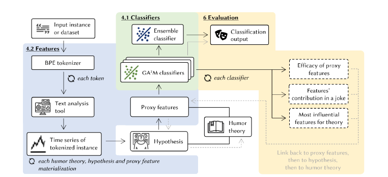
Figure 1: Architecture of the THInC framework (Figure from Marez et al.)[1]
The most significant difficulty researchers have had with incorporating humor into AI is determining how to distill it into a computable format. Due to their vague nature, a theory can be arbitrarily stretched to fit any number of jokes. This poses a problem for anyone attempting to detect humor. How can one convert something as qualitative as humor to numerical values?
Marez et al. took a clever approach to encoding the theories. Jokes usually work in a linear manner, with a clear start and end to a joke, so they decided to transform the text into a time series. By tokenizing the sentence and using tools like TweetNLP’s sentiment analysis and emotion recognition models, the researchers developed a way to map how different emotions changed over time in a given sentence.
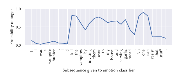
Figure 2: Time series representation of Anger in a joke (Figure from Marez et al.)[1]
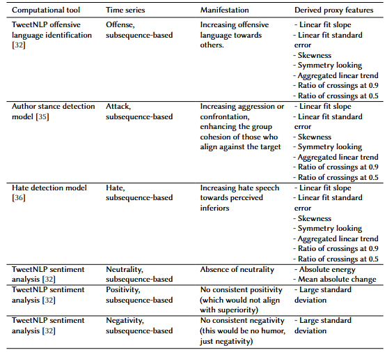
From here, they generated several hypotheses to serve as “manifestations” of the humor theories they could use to create features. For example, a hypothesis/manifestation of the relief theory is an increase in optimism within the joke. Using the manifestation, they would find ways to convert that to numerical proxy features, which serve as a representation of the humor theory and the hypothesis. The example of increasing optimism would be represented by the slope of the linear fit of the time series. The group would define several hypotheses for every humor theory, convert each to a proxy feature, and use those proxy features to train each model.
For example, the model for the superiority theories would use the proxy features representing offense and attack. In contrast, the relief theory would use features representing a change in optimism or joy.
Figure 3: Proposed Hypotheses For the Superiority Theory (Figure from Marez et al.)[1]
Methods
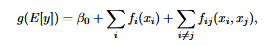
Once the proxy features were calculated, Marez et al. used a Generalized Additive Model (GAM) with pairwise interactions (AKA a GA2M) model to interpretively classify humor.
A Generalized Additive Model (GAM) is an extension of generalized linear models (GLMs) that allows for non-linear relationships between the features and the output[3]. Rather than sum linear terms, a GAM sums up nonlinear functions such as splines and polynomials to get a final data fit. A good comparison would be a scoreboard. Each function in the GAM is a separate player that individually contributes or detracts from the overall score. The final score is the prediction the model makes.
A GA2M extends the standard GAM by incorporating pairwise terms, enabling it to capture not just how individual features contribute to the predictions but also how pairs of features interact with each other [1]. Looking back to the scoreboard example, a GA2M would be what happens if we included teamwork in the mix, where features can “interact” with each other.
Figure 4: Equation for GA2M (Figure from Nijholt et al.)[2]
The specific GAM chosen by Marez et al. is the EBM(Explainable Boosting Machine) from the InterpretML Library. An EBM applies gradient boosting to each feature to significantly improve the performance of a model. For more details, refer to the InterpretML documentation here or the explanation by its developer here
Why GA2M?
Interpretability: GAMs and by extension GA2Ms allow for interpretability on the feature level. An outside party would be able to see the impacts that individual proxy features have on the results.
Flexibility: By incorporating interaction terms, GA2M enables the exploration of relationships between different features. This is particularly useful in humor classification. For example, it can help us understand how optimism relates to positivity when following the relief theory.
At the end of the training, the group can then combine the results from each of the classifiers to determine the relative impact of each emotion and each humor theory on whether or not a phrase will be perceived as a joke.
Results
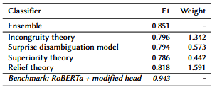
The model was remarkably accurate, with the combined model having an F1 score of 85%, indicating that the model has high precision and recall. The individual models also performed reasonably well, with F1 scores ranging from 79 to 81.
Figure 4: F1 scores for ensemble and individual classifiers (Figure from Marez et al.)[1]
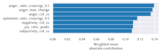
Furthermore, the model keeps this score while being very interpretable. Below, we can see each proxy feature’s contribution to the result.
Figure 5: Individual contributions of Emotions with the Incongruity theory (Figure from Marez et. al)[1]
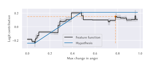
A GA2M also allows for feature-level analysis of contribution where the feature function can be graphed to determine the contribution of a feature in relation to its value. Figure 6 below shows an example of this. The graph shows how an increased anger change also contributes to a higher likelihood of being classified as a joke under the incongruity theory.
Figure 6: Figure function graph for incongruity theory (Figure from Marez et al.)[1]
Despite the framework’s incredible performance, the proxy features could be improved. These include revisiting and revising existing humor theories and making the proxy features more robust to the noise present in the text.
Conclusion
Humor is still a nebulous aspect of the human experience. Our current humor theories are still vague and too flexible, which can be annoying to convert to a computational model. The THInC framework is a promising step in the right direction. There’s no doubt that the framework has its issues, but many of those flaws stem from the unclear nature of humor itself. It’s hard to get a machine to know humor when humans still haven’t figured it out. The integration of sentiment analysis and emotion recognition into humor classification demonstrates a novel approach to incorporating humor theories into humor detection and the use of a GA2M is an ingenious way to incorporate the many nuances of humor into its function.
[1] De Marez, V., Winters, T., & Terryn, A. R. (2024). THInC: A Theory-Driven Framework for Computational humor Detection. arXiv preprint arXiv:2409.01232.
[2] A. Nijholt, O. Stock, A. Dix, J. Morkes, humor modeling in the interface, in: CHI’03 extended abstracts on Human factors in computing systems, 2003, pp. 1050–1051
[3] Hastie, T., Tibshirani, R., & Friedman, J. H. (2009). The Elements of Statistical Learning: Data Mining, Inference, and Prediction (2nd ed.). New York, Springer
We use cookies on our website to give you the most relevant experience by remembering your preferences and repeat visits. By clicking “Accept”, you consent to the use of ALL the cookies.
This website uses cookies to improve your experience while you navigate through the website. Out of these, the cookies that are categorized as necessary are stored on your browser as they are essential for the working of basic functionalities of the website. We also use third-party cookies that help us analyze and understand how you use this website. These cookies will be stored in your browser only with your consent. You also have the option to opt-out of these cookies. But opting out of some of these cookies may affect your browsing experience.
Necessary cookies are absolutely essential for the website to function properly. These cookies ensure basic functionalities and security features of the website, anonymously.
Cookie
Duration
Description
cookielawinfo-checkbox-analytics
11 months
This cookie is set by GDPR Cookie Consent plugin. The cookie is used to store the user consent for the cookies in the category "Analytics".
cookielawinfo-checkbox-functional
11 months
The cookie is set by GDPR cookie consent to record the user consent for the cookies in the category "Functional".
cookielawinfo-checkbox-necessary
11 months
This cookie is set by GDPR Cookie Consent plugin. The cookies is used to store the user consent for the cookies in the category "Necessary".
cookielawinfo-checkbox-others
11 months
This cookie is set by GDPR Cookie Consent plugin. The cookie is used to store the user consent for the cookies in the category "Other.
cookielawinfo-checkbox-performance
11 months
This cookie is set by GDPR Cookie Consent plugin. The cookie is used to store the user consent for the cookies in the category "Performance".
viewed_cookie_policy
11 months
The cookie is set by the GDPR Cookie Consent plugin and is used to store whether or not user has consented to the use of cookies. It does not store any personal data.
Functional cookies help to perform certain functionalities like sharing the content of the website on social media platforms, collect feedbacks, and other third-party features.
Performance cookies are used to understand and analyze the key performance indexes of the website which helps in delivering a better user experience for the visitors.
Analytical cookies are used to understand how visitors interact with the website. These cookies help provide information on metrics the number of visitors, bounce rate, traffic source, etc.
Advertisement cookies are used to provide visitors with relevant ads and marketing campaigns. These cookies track visitors across websites and collect information to provide customized ads.