Tag: tech

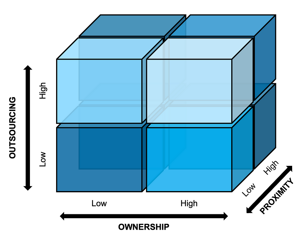
The interplay between ownership, outsourcing, and remote work

As we enter 2025, artificial intelligence (AI) is taking center stage at companies across industries. Faced with the twin challenges of acting decisively in the short run (or at least appearing to do so to reassure various stakeholders) and securing a prosperous future for the company in the long run, executives may be compelled to launch strategic AI initiatives. The aims of these initiatives can range from upgrading the company’s technical infrastructure and harvesting large amounts of high-quality training data, to improving the productivity of employees and embedding AI across the company’s products and services to offer greater value to customers.

Organizing in the right way is crucial to the successful implementation of such AI initiatives and can depend on a company’s particular context, e.g., budgetary constraints, skills of existing employees, and path dependency due to previous activities. This article takes a closer look at the interplay between three key dimensions of organizing for AI in today’s complex world: ownership, outsourcing, and proximity. We will see how different combinations of these dimensions could manifest themselves in the AI initiatives of various companies, compare pros and cons, and close with a discussion of past, present, and future trends.

Note: All figures and tables in the following sections have been created by the author of this article.

Guiding Framework

Figure 1 below visualizes the interplay between the three dimensions of ownership, outsourcing, and proximity, and this will serve as the guiding framework for the rest of the article.

The ownership dimension reflects whether the team implementing a given initiative will also own the initiative going forward, or instead act as consultants to another team that will take over long-term ownership. The outsourcing dimension captures whether the team for the initiative is primarily staffed with the company’s own employees or external consultants. Lastly, the proximity dimension considers the extent to which team members are co-located or based remotely; this dimension has gained in relevance following the wide experimentation with remote work by many companies during the global COVID-19 pandemic and throughout the escalation of geopolitical tensions around the world since then.

Although Figure 1 depicts the dimensions as clear-cut dichotomies for the sake of simplicity (e.g., internal versus external staffing), they of course have shades of gray in practice (e.g., hybrid approaches to staffing, industry partnerships). In their simplified form, the boxes in Figure 1 suggest eight possible ways of organizing for AI initiatives in general; we can think of these as high-level organizational archetypes. For example, to build a flagship AI product, a company could opt for an internally staffed, co-located team that takes full long-term ownership of the product. Alternatively, the company might choose to set up an outsourced, globally dispersed team, to benefit from a broader pool of AI talent.

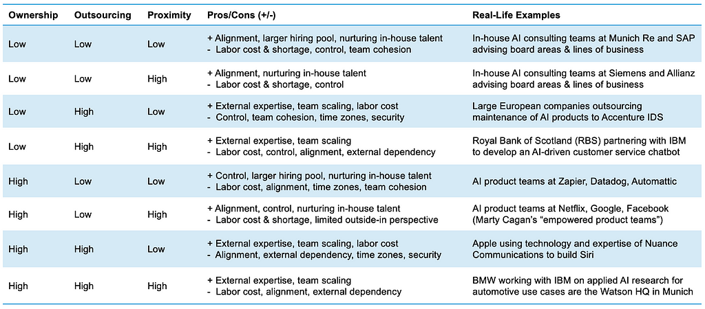
Organizational Archetypes for AI

Table 1 below provides an overview of the eight high-level organizational archetypes, including real-life examples from companies around the world. Each archetype has some fundamental pros and cons that are largely driven by the interplay between the constituent dimensions.

Archetypes with high ownership tend to offer greater long-term accountability, control, and influence over the outcomes of the AI initiative when the level of outsourcing is minimal, since in-house team members typically have more “skin in the game” than external consultants. But staffing AI experts internally can be expensive, and CFOs may be especially wary of this given the uncertain return on investment (ROI) of many early AI initiatives. It may also be harder to flexibly allocate and scale the scarce supply of in-house experts across different initiatives.

Meanwhile, archetypes that combine a high level of outsourcing and low proximity can allow AI initiatives to be implemented more cost-effectively, flexibly, and with greater infusion of specialized external expertise (e.g., a US-based company building an AI product with the help of externally sourced AI experts residing in India), but they come with cons such as external dependencies that can result in vendor lock-in and lower retention of in-house expertise, security risks leading to reduced protection of intellectual property, and difficulties in collaborating effectively with geographically dispersed external partners, potentially across time zones that are inconveniently far apart.

Current and Future Trends

As the real-life examples listed in Table 1 show, companies are already trying out different organizational archetypes. Given the trade-offs inherent to each archetype, and the nascent state of AI adoption across industries overall, the jury is still out on which archetypes (if any) lead to more successful AI initiatives in terms of ROI, positive market signaling, and the development of a sustained competitive advantage.

However, some archetypes do seem to be more common today — or at least have more vocal evangelists — than others. The combination of high ownership, low outsourcing, and high proximity (e.g., core AI products developed by co-located in-house teams) has been the preferred archetype of successful tech companies like Google, Facebook, and Netflix, and influential product coaches such as Marty Cagan have done much to drive its adoption globally. Smaller AI-first companies and startups may also opt for this organizational archetype to maximize control and alignment across their core AI products and services. But all these companies, whether large or small, tend to show strong conviction about the value that AI can create for their businesses, and are thus more willing to commit to an archetype that can require more funding and team discipline to execute properly than others.

For companies that are earlier in their AI journeys, archetypes involving lower ownership of outcomes, and greater freedom of outsourcing and remote staffing tend to be more attractive today; this may in part be due to a combination of positive signaling and cautious resource allocation that such archetypes afford. Although early-stage companies may not have identified a killer play for AI yet, they nonetheless want to signal to stakeholders (customers, shareholders, Wall Street analysts, and employees) that they are alert to the strategic significance of AI for their businesses, and ready to strike should a suitable opportunity present itself. At the same time, given the lack of a killer play and the inherent difficulty of estimating the ROI of early AI initiatives, these companies may be less willing to place large sticky bets involving the ramp-up of in-house AI staff.

Looking to the future, a range of economic, geopolitical, and technological factors will likely shape the options that companies may consider when organizing for AI. On the economic front, the cost-benefit analysis of relying on external staffing and taking ownership of AI initiatives may change. With rising wages in countries such as India, and the price premium attached to high-end AI services and expertise, the cost of outsourcing may become too high to justify any benefits. Moreover, for companies like Microsoft that prioritize the ramp-up of internal AI R&D teams in countries like India, it may be possible to reap the advantages of internal staffing (alignment, cohesion, etc.) while benefiting from access of affordable talent. Additionally, for companies that cede ownership of complex, strategic AI initiatives to external partners, switching from one partner to another may become prohibitively expensive, leading to long-term lock-in (e.g., using the AI platform of an external consultancy to develop custom workflows and large-scale models that are difficult to migrate to more competitive providers later).

The geopolitical outlook, with escalating tensions and polarization in parts of Eastern Europe, Asia, and the Middle East, does not look reassuring. Outsourcing AI initiatives to experts in these regions can pose a major risk to business continuity. The risk of cyber attacks and intellectual property theft inherent to such conflict regions will also concern companies seeking to build a lasting competitive advantage through AI-related proprietary research and patents. Furthermore, the threat posed by polarized national politics in mature and stagnating Western economies, coupled with the painful lessons learned from disruptions to global supply chains during the COVID-19 pandemic, might lead states to offer greater incentives to reshore staffing for strategic AI initiatives.

Lastly, technologies that enable companies to organize for AI, and technologies that AI initiatives promise to create, will both likely inform the choice of organizational archetypes in the future. On the one hand, enabling technologies related to online video-conferencing, messaging, and other forms of digital collaboration have greatly improved the remote working experience of tech workers. On the other hand, in contrast to other digital initiatives, AI initiatives must navigate complex ethical and regulatory landscapes, addressing issues around algorithmic and data-related bias, model transparency, and accountability. Weighing the pros and cons, a number of companies in the broader AI ecosystem, such as Zapier and Datadog, have adopted a remote-first working model. The maturity of enabling technologies (increasingly embedded with AI), coupled with the growing recognition of societal, environmental, and economic benefits of fostering some level of remote work (e.g., stimulating economic growth outside big cities, reducing pollution and commute costs, and offering access to a broader talent pool), may lead to further adoption and normalization of remote work, and spur the development of best practices that minimize the risks while amplifying the advantages of low proximity organizational archetypes.

---

Organizing for AI was originally published in Towards Data Science on Medium, where people are continuing the conversation by highlighting and responding to this story.

You can’t afford to remain an AI-ignoramus, even if your product isn’t using an LLM

If you’re a Software Architect, or a Tech Lead, or really anyone senior in tech whose role includes making technical and strategic decisions, and you’re not a Data Scientist or Machine Learning expert, then the likelihood is that Generative AI and Large Language Models (LLMs) were new to you back in 2023.

AI was certainly new to me.

We all faced a fork in the road —should we invest the time and effort to learn GenAI or continue on our jolly way?

At first, since the products I’m working on are not currently using AI, I dipped my toes in the water with some high-level introductory training on AI, and then went back to my day job of leading the architecture for programmatic features and products. I reassured myself that we can’t all be experts in everything — the same way I’m not a computer vision expert, I don’t need to be an AI expert — and instead I should remain focused on high level architecture along with my core areas of expertise- cloud and security.

Did you face a similar decision recently?

I’m guessing you did.

I’m here to tell you that if you chose the path of LLM-semi-ignorance, you’re making a huge mistake.

Luckily for me, I was part of a team that won a global hackathon for our idea around using AI for improving organizational inclusivity, and that kicked off a POC using GenAI. That then led to co-authoring a patent centered around LLM fine-tuning. I was bothered by my ignorance when AI terms flew around me, and started investing more in my own AI ramp-up, including learning from the experts within my organization, and online courses which went beyond the introductory level and into the architecture. Finally it all clicked into place. I’m still not a data scientist, but I can understand and put together a GenAI based architecture. This enabled me to author more patents around GenAI, lead an experimental POC using an LLM and AI agents, and participate in a GenAI hackathon.

What I learned from this experience is that GenAI is introducing entirely new paradigms, which are diametrically opposed to everything I knew until now. Almost every single fact from my computer science degrees, academic research, and work experience is turned on its head when I’m designing a GenAI system.

GenAI means solving problems using non-deterministic solutions. We got used to programmatic and deterministic algorithms, allowing us to predict and validate inputs against outputs. That’s gone. Expect different results each time, start thinking about a percentage of success vs absolute correctness.

GenAI means results are not linear to development effort investment. Some problems are easy to solve with a simple prompt, others require prior data exploration and complex chains of multiple agentic AI workflows, and others require resource heavy fine tuning. This is very different than assessing a requirement, translating it to logical components and being able to provide an initial decomposition and effort assessment. When we use an LLM, in most cases, we have to get our hands dirty and try it out before we can define the software design.

As a software architect, I’ve begun assessing tradeoffs around using GenAI vs sticking with class programmatic approaches, and then digging deeper to analyze tradeoffs within GenAI — Should we using fine tuning vs. RAG, where is an AI agent needed? Where is further abstraction and multi-agents needed? Where should we combine programmatic pre-processing with an LLM?

For every single one of these architectural decision points- GenAI understanding is a must.

I became a Software Architect after over a decade of experience as a Software Engineer, developing code in multiple languages and on multiple tech stacks, from embedded to mobile to SaaS. I understand the nuts and bolts of programmatic code, and even though I’m not writing code anymore myself, I rely on my software development background both for making high level decisions and for delving into the details when necessary. If as tech leaders we don’t ensure that we gain equivalent knowledge and hands-on experience in the field of GenAI, we won’t be able to lead the architecture of modern systems.

In other words — I realized that I cannot be a good Software Architect, without knowing GenAI. The same way I can’t be a good Software Architect if I don’t understand topics such as algorithms, complexity, scaling; architectures such as client-server, SaaS, relational and non-relational data bases; and other computer science foundations.

GenAI has become foundational to computer engineering. GenAI is no longer a niche sub-domain that can be abstracted away and left to Subject Matter Experts. GenAI means new paradigms and new ways of thinking about software architecture and design. And I don’t think any Software Architect or Tech Leader can reliably make decisions without having this knowledge.

It could be that the products and projects you lead will remain AI free. GenAI is not a silver bullet, and we need to ensure we don’t replace straightforward automation with AI when it’s not needed and even detrimental. All the same, we need to be able to at least assess this decision knowledgeably, every time we face it.

I’m going to end with some positive news for Software Architects — yes we all have to ramp-up and learn AI — but once we do, we’re needed!

As GenAI based tools become ever more complex, data science and AI expertise is not going to be enough — we need to architect and design these systems taking into account all those other factors we’ve been focused on until now — scale, performance, maintainability, good design and composability — there’s a lot that we can contribute.

But first we need to ensure we learn the new paradigms as GenAI transforms computer engineering — and make sure we’re equipped to continue to be technical decision makers in this new world.

---

Why Every Software Architect Needs to Learn GenAI was originally published in Towards Data Science on Medium, where people are continuing the conversation by highlighting and responding to this story.

A discussion around measuring error rates in IBM quantum processors, with code examples, using Qiskit

Quantum computing has made significant strides in recent years, with breakthroughs in hardware stability, error mitigation, and algorithm development bringing us closer to solving problems that classical computers cannot tackle efficiently. Companies and research institutions worldwide are pushing the boundaries of what quantum systems can achieve, transforming this once-theoretical field into a rapidly evolving technology. IBM has emerged as a key player in this space, offering IBM Quantum, a platform that provides access to state-of-the-art quantum processors (QPUs) with a qubit capacity in the hundreds. Through the open-source Qiskit SDK, developers, researchers, and enthusiasts can design, simulate, and execute quantum circuits on real quantum hardware. This accessibility has accelerated innovation while also highlighting key challenges, such as managing the error rates that still limit the performance of today’s quantum devices.

By leveraging the access to quantum processors available for free on the IBM platform, we propose to run a few quantum computations to measure the current level of quantum noise in basic circuits. Achieving a low enough level of quantum noise is the most important challenge in making quantum computing useful. Unfortunately, there is not a ton of material on the web explaining the current achievements. It is also not obvious what quantity we want to measure and how to measure it in practice.

In this blogpost,

• We will review some basics of quantum circuits manipulations in Qiskit.
• We will explain the minimal formalism to discuss quantum errors, explaining the notion of quantum state fidelity.
• We will show how to estimate the fidelity of states produced by simple quantum circuits.

To follow this discussion, you will need to know some basics about Quantum Information Theory, namely what are qubits, gates, measurements and, ideally, density matrices. The IBM Quantum Learning platform has great free courses to learn the basics and more on this topic.

Disclaimer: Although I am aiming at a decent level of scientific rigorousness, this is not a research paper and I do not pretend to be an expert in the field, but simply an enthusiast, sharing my modest understanding.

To start with, we need to install Qiskit tools

%pip install qiskit qiskit_ibm_runtime
%pip install 'qiskit[visualization]'

import qiskit
import qiskit_ibm_runtime

print(qiskit.version.get_version_info())
print(qiskit_ibm_runtime.version.get_version_info())

1.3.1
0.34.0

Running a quantum circuit and observing errors

Quantum computations consist in building quantum circuits, running them on quantum hardware and collecting the measured outputs.

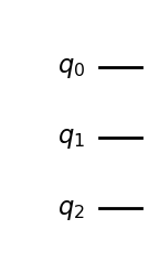
To build a quantum circuit, we start by specifying a number n of qubits for our circuits, where n can be as large as 127 or 156, depending on the underling QPU instance (see processor types). All n qubits are initialised in the |0⟩ state, so the initial state is |0 ⟩ⁿ . Here is how we initialise a circuit with 3 qubits in Qiskit.

from qiskit.circuit import QuantumCircuit

# A quantum circuit with three qubits
qc = QuantumCircuit(3)
qc.draw('mpl')

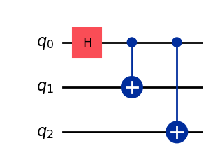
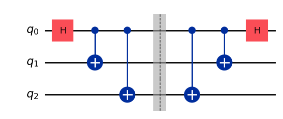
Next we can add operations on those qubits, in the form of quantum gates, which are unitary operations acting typically on one or two qubits. For instance let us add one Hadamard gate acting on the first qubit and two CX (aka CNOT) gates on the pairs of qubits (0, 1) and (0, 2).

# Hadamard gate on qubit 0.
qc.h(0)
# CX gates on qubits (0, 1) and (0, 2).
qc.cx(0, 1)
qc.cx(0, 2)

qc.draw('mpl')

We obtain a 3-qubit circuit preparing the state

To measure the output qubits of the circuit, we add a measurement layer

qc.measure_all()
qc.draw('mpl')

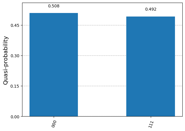
It is possible to run the circuit and to get its output measured bits as a simulation with StatevectorSampleror on real quantum hardware with SamplerV2 . Let us see the output of a simulation first.

from qiskit.primitives import StatevectorSampler
from qiskit.transpiler.preset_passmanagers import generate_preset_pass_manager
from qiskit.visualization import plot_distribution

sampler = StatevectorSampler()
pm = generate_preset_pass_manager(optimization_level=1)
# Generate the ISA circuit
qc_isa = pm.run(qc)
# Run the simulator 10_000 times
num_shots = 10_000
result = sampler.run([qc_isa], shots=num_shots).result()[0]
# Collect and plot measurements
measurements= result.data.meas.get_counts()
plot_distribution(measurements)

The measured bits are either (0,0,0) or (1,1,1), with approximate probability close to 0.5. This is precisely what we expect from sampling the 3-qubit state prepared by the circuit.

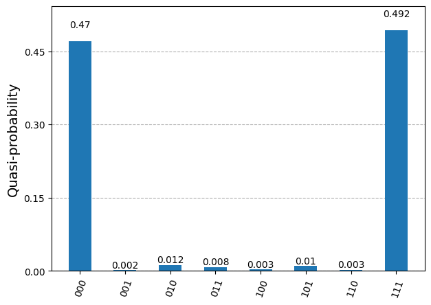
We now run the circuit on a QPU (see instructions on setting up an IBM Quantum account and retrieving your personal token)

from qiskit_ibm_runtime import QiskitRuntimeService
from qiskit_ibm_runtime import SamplerV2 as Sampler

service = QiskitRuntimeService(
    channel="ibm_quantum",
    token=<YOUR_TOKEN>, # use your IBM Quantum token here.
)
# Fetch a QPU to use
backend = service.least_busy(operational=True, simulator=False)
print(f"QPU: {backend.name}")
target = backend.target
sampler = Sampler(mode=backend)
pm = generate_preset_pass_manager(target=target, optimization_level=1)
# Generate the ISA circuit
qc_isa = pm.run(qc)
# Run the simulator 10_000 times
num_shots = 10_000
result = sampler.run([qc_isa], shots=num_shots).result()[0]
# Collect and plot measurements
measurements= result.data.meas.get_counts()
plot_distribution(measurements)

QPU: ibm_brisbane

The measured bits are similar to those of the simulation, but now we see a few occurrences of the bit triplets (0,0,1), (0,1,0), (1,0,0), (0,1,1), (1,0,1) and (1,1,0). Those measurements should not occur from sampling the 3-qubit state prepared by the chosen circuit. They correspond to quantum errors occurring while running the circuit on the QPU.

We would like to quantify the error rate somehow, but it is not obvious how to do it. In quantum computations, what we really care about is that the qubit quantum state prepared by the circuit is the correct state. The measurements which are not (0,0,0) or (1,1,1) indicate errors in the state preparation, but this is not all. The measurements (0,0,0) and (1,1,1) could also be the result of incorrectly prepared states, e.g. the state (|0,0,0⟩ + |0,0,1⟩)/√2 can produce the output (0,0,0). Actually, it seems very likely that a few of the “correct” measurements come from incorrect 3-qubit states.

To understand this “noise” in the state preparation we need the formalism of density matrices to represent quantum states.

Density matrices and state fidelity

The state of an n-qubit circuit with incomplete information is represented by a 2ⁿ× 2ⁿ positive semi-definite hermitian matrix with trace equal to 1, called the density matrix ρ. Each diagonal element corresponds to the probability pᵢ of measuring one of the 2ⁿ possible states in a projective measurement, pᵢ = ⟨ψᵢ| ρ |ψᵢ⟩. The off-diagonal elements in ρ do not really have a physical interpretation, they can be set to zero by a change of basis states. In the computational basis, i.e. the standard basis |bit₀, bit₁, …, bitₙ⟩, they encode the entanglement properties of the state. Vector states |ψ⟩ describing the possible quantum states of the qubits have density matrices ρ = |ψ⟩⟨ψ|, whose eigenvalues are all 0, except for one eigenvalue, which is equal to 1. They are called pure states. Generic density matrices represent probabilistic quantum states of the circuit and have eigenvalues between 0 and 1. They are called mixed states. To give an example, a circuit which is in a state |ψ₁⟩ with probability q and in a state |ψ₂⟩ with probability 1-q is represented by the density matrix ρ = q|ψ₁⟩⟨ψ₁| + (1-q)|ψ₂⟩⟨ψ₂|.

In real quantum hardware, qubits are subject to all kinds of small unknown interactions with the environment, leading to a “loss of information”. This is the source of an incoherent quantum noise. Therefore, when applying gates to qubits or even when preparing the initial state, the quantum state of qubits cannot be described by a pure state, but ends up in a mixed state, which we must describe with a density matrix ρ. Density matrices provide a convenient way to describe quantum circuits in isolation, abstracting the complex and unknown interactions with the environment.

To learn more about density matrix representation of quantum states, you can look at any quantum information course. The excellent Qiskit lecture on this topic is available on YouTube.

For a single qubit, the density matrix, in the computational basis (i.e. the basis {|0⟩, |1⟩}), is a 2×2 matrix

with p₀ = ⟨0|ρ|0⟩ the probability to measure 0, p₁ = 1 — p₀ = ⟨1|ρ|1⟩ the probability to measure 1, and c is a complex number bounded by |c|² ≤ p₀p₁. Pure states have eigenvalues 0 and 1, so their determinant is zero, and they saturate the inequality with |c|² = p₀p₁.

In the following, we will consider quantum circuits with a few qubits and we will be interested in quantifying how close the output state density matrix ρ is from the expected (theoretical) output density matrix ρ₀. For a single qubit state, we could think about comparing the values of p₀, p₁ and c, provided we are able to measure them, but in a circuit with more qubits and a larger matrix ρ, we would like to come up with a single number quantifying how close ρ and ρ₀ are. Quantum information theory possesses such quantity. It is called state fidelity and it is defined by the slightly mysterious formula

The state fidelity F is a real number between 0 an 1, 0 ≤ F ≤ 1, with F = 1 corresponding to having identical states ρ = ρ₀ , and F = 0 corresponding to ρ and ρ₀ having orthogonal images. Although it is not so obvious from the definition, it is a symmetric quantity, F(ρ,ρ₀) = F(ρ₀,ρ).

In quantum circuit computations, the expected output state ρ₀ is always a pure state ρ₀ = |ψ₀⟩⟨ψ₀| and, in this case, the state fidelity reduces to the simpler formula

which has the desired interpretation as the probability for the state ρ to be measured in the state |ψ₀⟩ (in a hypothetical experiment implementing a projective measurement onto the state |ψ₀⟩ ).

In the noise-free case, the produced density matrix is ρ = ρ₀ = |ψ₀⟩⟨ψ₀| and the state fidelity is 1. In the presence of noise the fidelity decreases, F < 1.

In the remainder of this discussion, our goal will be to measure the state fidelity F of simple quantum circuit in Qiskit, or, more precisely, to estimate a lower bound F̃ < F.

State fidelity estimation in quantum circuits

To run quantum circuits on QPUs and collect measurement results, we define the function run_circuit .

def run_circuit(
        qc: QuantumCircuit, 
        service: QiskitRuntimeService = service, 
        num_shots: int = 100,
    ) -> tuple[dict[str, int], QuantumCircuit]:
    """Runs the circuit on backend 'num_shots' times. Returns the counts of 
    measurements and the ISA circuit."""
    # Fetch an available QPU
    backend = service.least_busy(operational=True, simulator=False)
    target = backend.target
    pm = generate_preset_pass_manager(target=target, optimization_level=1)
    
    # Add qubit mesurement layer and compute ISA circuit
    qc_meas = qc.measure_all(inplace=False)
    qc_isa = pm.run(qc_meas)

    # Run the ISA circuit and collect results
    sampler = Sampler(mode=backend)
    result = sampler.run([qc_isa], shots=num_shots).result()
    dist = result[0].data.meas.get_counts()

    return dist, qc_isa

The ISA (Instruction Set Architecture) circuit qc_isa returned by this function is essentially a rewriting of the provided circuit in terms of the physical gates available on the QPU, called basis gates. This is the circuit that is actually constructed and run on the hardware.

Note: The run_circuit function starts by fetching an available QPU. This is convenient to avoid waiting too long for the computation to be processed. However this also means that we use different QPUs each time we call the function. This is not ideal, as it is possible that different QPUs have different level of quantum noise. However, in practice, the fetched QPUs all turned out to be in the Eagle family and we present noise estimation only for this QPU family. To keep our analysis simple, we just assume that the level of quantum noise among the possible QPU instances is stable. The interested reader could try to find whether there are differences between instances.

Bare |0⟩ state

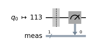
Let us start with the simplest circuit, which comprises only an initialised qubit |0⟩ without any gate operation.

# A quantum circuit with a single qubit |0>
qc = QuantumCircuit(1)
dist, qc_isa = run_circuit(qc, num_shots=100_000)
qc_isa.draw(output="mpl", idle_wires=False, style="iqp")

import numpy as np

def print_results(dist: dict[str, int]) -> None:
    print(f"Measurement counts: {dist}")
    num_shots = sum([dist[k] for k in dist])
    for k, v in dist.items():
        p = v / num_shots
        # 1% confidence interval estimate for a Bernoulli variable
        delta = 2.575 * np.sqrt(p*(1-p)/num_shots)
        print(f"p({k}): {np.round(p, 4)}  ± {np.round(delta, 4)}")

print_results(dist)

Measurement counts: {'0': 99661, '1': 339}
p(0) = 0.9966 ± 0.0005
p(1) = 0.0034 ± 0.0005

We get a small probability, around 0.3%, to observe the incorrect result 1. The interval estimate “± 0.0005” refers to a 1% confidence interval estimate for a Bernoulli variable.

The fidelity of the output state ρ, relative to the ideal state |0⟩, is F = ⟨0|ρ|0⟩ = p₀. We have obtained an estimate of 0.9966 ± 0.0005 for p₀ from the repeated measurements of the circuit output state. But the measurement operation is a priori imperfect (it has its own error rate). It may add a bias to the p₀ estimate. We assume that these measurement errors tend to decrease the estimated fidelity by incorrect measurements of |0⟩ states. In this case, the estimated p₀ will be a lower bound on the true fidelity F:

F > F̃ = 0.9966 ± 0.0005

Note: We have obtained estimated probabilities p₀, p₁ for the diagonal components of the single-qubit density matrix ρ. We also have an estimated bound on the off-diagonal component |c| < √(p₀ p₁) ~ 0.06. To get an actual estimate for c, we would need to run a circuit some gates and design a more complex reasoning.

Basis gates

Qiskit offers a large number of quantum gates encoding standard operations on one or two qubits, however all these gates are encoded in the QPU hardware with combinations of a very small set of physical operations on the qubits, called basis gates.

There are three single-qubit basis gates: X, SX and RZ(λ) and one two-qubit basis gate: ECR. All other quantum gates are constructed from these building blocks. The more basis gates are used in a quantum circuit, the larger is the quantum noise. We will analyse the noise resulting from applying these basis gates in isolation, when possible, or with a minimal number of basis gates, to get a sense of quantum noise in the current state of QPU computations.

X gate

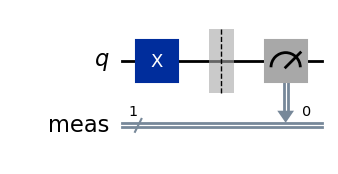
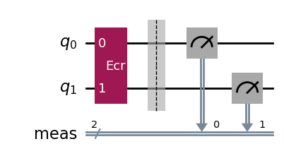
We consider the circuit made of a single qubit and an X gate. The output state, in the absence of noise, is X|0⟩ = |1⟩.

# Quantum circuit with a single qubit and an X gate. 
# Expected output state X|0> = |1>.
qc = QuantumCircuit(1)
qc.x(0)

dist, qc_isa = run_circuit(qc, num_shots=100_000)
qc_isa.draw(output="mpl", idle_wires=False, style="iqp")

print_results(dist)

Measurement counts: {'1': 99072, '0': 928}
p(0) = 0.0093 ± 0.0008
p(1) = 0.9907 ± 0.0008

The state fidelity of the output state ρ, relative to the ideal state |1⟩, is

F = ⟨1|ρ|1⟩ = p₁ > F̃ = 0.9907 ± 0.0008

where we assumed again that the measurement operation lower the estimated fidelity and we get a lower bound F̃ on the fidelity.

We observe that the fidelity is (at least) around 99.1%, which is a little worse than the fidelity measured without the X gate. Indeed, adding a gate to the circuit should add noise, but there can be another effect contributing to the degradation of the fidelity, which is the fact that the |1⟩ state is a priori less stable than the |0⟩ state and so the measurement of a |1⟩ state itself is probably more noisy. We will not discuss the physical realisation of a qubit in IBM QPUs, but one thing to keep in mind is that the |0⟩ state has lower energy than the |1⟩ state, so that it is quantum mechanically more stable. As a result, the |1⟩ state can decay to the |0⟩ state through interactions with the environement.

SX gate

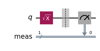
We now consider the SX gate, i.e. the “square-root X” gate, represented by the matrix

It transforms the initial qubit state |0⟩ into the state

# Quantum circuit with a single qubit and an SX gate. 
qc = QuantumCircuit(1)
qc.sx(0)

dist, qc_isa = run_circuit(qc, num_shots=100_000)
qc_isa.draw(output="mpl", idle_wires=False, style="iqp")

print_results(dist)

Measurement counts: {'1': 50324, '0': 49676}
p(0) = 0.4968 ± 0.0041
p(1) = 0.5032 ± 0.0041

We observe roughly equal distributions of zeros and ones, which is as expected. But we face a problem now. The state fidelity cannot be computed from these p₀ and p₁ estimates. Indeed, the fidelity of the output state ρ, relative to the ideal output state SX|0⟩ is

Therefore, to get an estimate of F, we also need to measure c, or rather its imaginary part Im(c). Since there is no other measurement we can do on the SX gate circuit, we need to consider a circuit with more gates to evaluate F, but more gates also means more sources of noise.

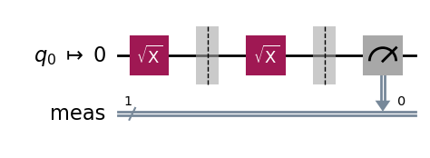
One simple thing we can do is to add either another SX gate or an SX⁻¹ gate. In the former case, the full circuit implements the X operation and the expected final state |1⟩, while in the latter case, the full circuit implements the identity operation and the expected final state is |0⟩.

Let us consider the case of adding an SX gate: the density matrix ρ produced by the first SX gate gets transformed into

leading to p’₁ = 1/2— Im(c) = F, in the ideal case when the second SX gate is free of quantum noise. In practice the SX gate is imperfect and we can only measure p’₁ = 1/2 — Im(c) — δp = F — δp, where δp is due to the noise from the second SX gate. Although it is theoretically possible that the added noise δp combines with the noise introduced by the first SX gate and results in a smaller combined noise, we will assume that no such “happy” cancelation happens, so that we have δp>0. In this case, p’₁ < F gives us a lower bound on the state fidelity F.

qc = QuantumCircuit(1)
qc.sx(0)
qc.barrier() # Prevents simplification of the circuit during transpilation.
qc.sx(0)

dist, qc_isa = run_circuit(qc, num_shots=100_000)

print_results(dist)

Measurement counts: {'1': 98911, '0': 1089}
p(1): 0.9891  ± 0.0008
p(0): 0.0109  ± 0.0008

We obtain a lower bound F > p’₁ = 0.9891 ± 0.0008, on the fidelity of the output state ρ for the SX-gate circuit, relative to the ideal output state SX|0⟩.

We could have considered the two-gate circuit with an SX gate followed by an SX⁻¹ gate instead. The SX⁻¹ gate is not a basis gate. It is implemented in the QPU as SX⁻¹ = RZ(-π) SX RZ(-π). We expect this setup to add more quantum noise due the presence of more basis gates, but in practice we have measured a higher (better) lower bound F̃. The interested reader can check this as an exercise. We believe this is due to the fact that the unwanted interactions with the environment tend to bring the qubit state to the ground state |0⟩, improving incorrectly the lower bound estimate, so we do not report this alternative result.

RZ(λ) gate

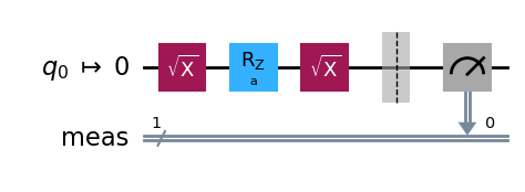
Next we consider the RZ(λ) gate. The RZ(λ) gate is a parametrised gate implementing a rotation around the z-axis by an angle λ/2.

Its effect on the initial qubit |0⟩ is only to multiply it by a phase exp(-iλ/2), leaving it in the same state. In general, the action of RZ(λ) on the density matrix of a single qubit is to multiply the off-diagonal coefficient c by exp(iλ), leaving the p₀ and p₁ values of the state unchanged. To measure a non-trivial effect of the RZ(λ) gate, one needs to consider circuits with more gates. The simplest is to consider the circuit composing the three gates SX, RZ(λ) and SX, preparing the state

The expected p(0) and p(1) values are

Qiskit offers the possibility to run parametrised quantum circuits by specifying an array of parameter values, which, together with the ISA circuit, define a Primitive Unified Bloc (PUB). The PUB is then passed to the sampler to run the circuit with all the specified parameter values.

from qiskit.primitives.containers.sampler_pub_result import SamplerPubResult

def run_parametrised_circuit(
        qc: QuantumCircuit, 
        service: QiskitRuntimeService = service, 
        params: np.ndarray | None = None,
        num_shots: int = 100,
    ) -> tuple[SamplerPubResult, QuantumCircuit]:
    """Runs the parametrised circuit on backend 'num_shots' times. 
    Returns the PubResult and the ISA circuit."""
    # Fetch an available QPU
    backend = service.least_busy(operational=True, simulator=False)
    target = backend.target
    pm = generate_preset_pass_manager(target=target, optimization_level=1)
    
    # Add mesurement layer
    qc_meas = qc.measure_all(inplace=False)
    # Define ISA circuit and PUB
    pm = generate_preset_pass_manager(target=target, optimization_level=1)
    qc_isa = pm.run(qc_meas)
    sampler_pub = (qc_isa, params)
    
    # Run the circuit
    result = sampler.run([sampler_pub], shots=num_shots).result()
    return result[0], qc_isa

from qiskit.circuit import Parameter

# Circuit preparing the state SX.RZ(a).SX|0> = sin(a/2)|0> + cos(a/2)|1>.
qc = QuantumCircuit(1)
qc.sx(0)
qc.rz(Parameter("a"), 0)
qc.sx(0)

# Define parameter range
params = np.linspace(0, 2*np.pi, 21).reshape(-1, 1)
# Run parametrised circuit
pub_result, qc_isa = run_parametrised_circuit(qc, params=params, num_shots=10_000)

qc_isa.draw(output="mpl", idle_wires=False, style="iqp")

bit_array = pub_result.data.meas.bitcount()
print(f"bit_array shape: {bit_array.shape}")
p0 = (bit_array.shape[1] - bit_array.sum(axis=1)) / bit_array.shape[1]
p1 = bit_array.sum(axis=1) / bit_array.shape[1]
print(f"p(0): {p0}")
print(f"p(1): {p1}")

bit_array shape: (21, 10000)
p(0): [0.0031 0.0265 0.095  0.2095 0.3507 0.4969 0.6567 0.7853 0.9025 0.9703
 0.9983 0.976  0.901  0.7908 0.6543 0.5013 0.3504 0.2102 0.0982 0.0308
 0.0036]
p(1): [0.9969 0.9735 0.905  0.7905 0.6493 0.5031 0.3433 0.2147 0.0975 0.0297
 0.0017 0.024  0.099  0.2092 0.3457 0.4987 0.6496 0.7898 0.9018 0.9692
 0.9964]

import matplotlib.pyplot as plt

x = params/(2*np.pi)
plt.scatter(x, p0)
plt.scatter(x, p1)
plt.plot(x, np.sin(np.pi*x)**2, linestyle="--")
plt.plot(x, np.cos(np.pi*x)**2, linestyle="--")
plt.xlabel("λ/2π")
plt.ylabel("Estimated probabilities")
plt.legend(["p(0)", "p(1)", "sin(λ/2)^2", "cos(λ/2)^2"])
plt.show()

We see that the estimated probabilities (blue and orange dots) agree very well with the theoretical probabilities (blue and orange lines) for all tested values of λ.

Here again, this does not give us the state fidelity. We can give a lower bound by adding another sequence of gates SX.RZ(λ).SX to the circuit, bringing back the state to |0⟩. As in the case of the SX gate of the previous section, the estimated F̃ := p’₀ from this 6-gate circuit gives us a lower bound on the fidelity of the F of the 3-gate circuit, assuming the extra gates lower the output state fidelity.

Let us compute this lower bound F̃ for one value, λ = π/4.

# Circuit implementing SX.RZ(π/4).SX.SX.RZ(π/4).SX|0> = |0>
qc = QuantumCircuit(1)
qc.sx(0)
qc.rz(np.pi/4, 0)
qc.sx(0)
qc.barrier()  # Prevents circuit simplifications.
qc.sx(0)
qc.rz(np.pi/4, 0)
qc.sx(0)

dist, qc_isa = run_circuit(qc, num_shots=100_000)
qc_isa.draw(output="mpl", idle_wires=False, style="iqp")

dist = pub_result.data.meas.get_counts()
print_results(dist)

Measurement counts: {'0': 99231, '1': 769}
p(0): 0.9923  ± 0.0007
p(1): 0.0077  ± 0.0007

We find a pretty high lower bound estimate F̃ = 0.9923 ± 0.0007.

Digression: a lower bound estimate procedure

The above case showed that we can estimate a lower bound on the fidelity F of the output state of a circuit by extending the circuit with its inverse operation and measuring the probability of getting the initial state back.

Let us consider an n-qubit circuit preparing the state |ψ⟩ = U|0,0, … ,0⟩. The state fidelity of the output density matrix ρ is given by

U⁻¹ρU is the density matrix of the circuit composed of a (noisy) U gate and a noise-free U⁻¹ gate. F is equal to the fidelity of the |0,0, …, 0⟩ state of this 2-gate circuit. If we had such a circuit, we could sample it and measure the probability of (0, 0, …, 0) as the desired fidelity F.

In practice we don’t have a noise-free U⁻¹ gate, but only a noisy U⁻¹ gate. By sampling this circuit (noisy U, followed by noisy U⁻¹) and measuring the probability of the (0, 0, …, 0) outcome, we obtain an estimate F̃ of F — δp, with δp the noise overhead added by the U⁻¹ operation (and the measurement operation). Under the assumption δp>0, we obtain a lower bound F > F̃. This assumption is not necessarily true because the noisy interactions with the environment likely tend to bring the qubits to the ground state |0,0, …, 0⟩, but for “complex enough” operations U, this effect should be subdominant relative to the noise introduced by the U⁻¹ operation. We have used this approach to estimate the fidelity in the SX.RZ(λ).SX circuit above. We will use it again to estimate the fidelity of the ECR-gate and the 3-qubit state from the initial circuit we considered.

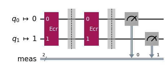
ECR gate

The ECR gate (Echoed Cross-Resonance gate) is the only two-qubit basis gate in the Eagle family of IBM QPUs (other families support the CZ or CX gate instead, see tables of gates). It is represented in the computational basis by the 4×4 matrix

Its action on the initial 2-qubit state is

The measurements of a noise-free ECR gate circuit are (0,1) with probability 1/2 and (1,1) with probability 1/2. The outcome (0,0) and (1,0) are not possible in the noise-free circuit.

qc = QuantumCircuit(2)
qc.ecr(0, 1)
dist, qc_isa = run_circuit(qc, num_shots=100_000)

qc_isa.draw(output="mpl", idle_wires=False, style="iqp")

print_results(dist)

Measurement counts: {'11': 49254, '01': 50325, '00': 239, '10': 182}
p(11): 0.4925  ± 0.0041
p(01): 0.5032  ± 0.0041
p(00): 0.0024  ± 0.0004
p(10): 0.0018  ± 0.0003

We observe a distribution of measured classical bits roughly agreeing with the expected ideal distribution, but the presence of quantum errors is revealed by the presence of a few (0,0) and (1, 0) outcomes.

The fidelity of the output state ρ is given by

As in the case of the SX-gate circuit, we cannot directly estimate the fidelity of the ρ state prepared by the ECR-gate circuit by measuring the output bits of the circuit, since it depends on off-diagonal terms in the ρ matrix.

Instead we can follow the procedure described in the previous section and estimate a lower bound on F by considering the circuit with an added ECR⁻¹ gate. Since ECR⁻¹ = ECR, we consider a circuit with two ECR gates.

qc = QuantumCircuit(2)
qc.ecr(0, 1)
qc.barrier()  # Prevents circuit simplifications.
qc.ecr(0, 1)
dist, qc_isa = run_circuit(qc, num_shots=100_000)
qc_isa.draw(output="mpl", idle_wires=False, style="iqp")

print_results(dist)

Measurement counts: {'00': 99193, '01': 153, '10': 498, '11': 156}
p(00): 0.9919  ± 0.0007
p(01): 0.0015  ± 0.0003
p(10): 0.005  ± 0.0006
p(11): 0.0016  ± 0.0003

We find the estimated lower bound F > 0.9919 ± 0.0007 on the ρ state prepared by the ECR-gate circuit.

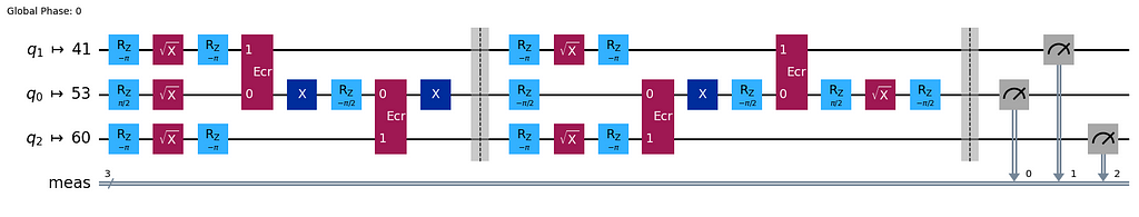
3-qubit state fidelity

To close the loop, in our final example, let us compute a lower bound on the state fidelity of the 3-qubit state circuit which we considered first. Here again, we add the inverse operation to the circuit, bringing back the state to |0,0,0⟩ and measure the circuit outcomes.

qc = QuantumCircuit(3)
qc.h(0)
qc.cx(0, 1)
qc.cx(0, 2)
qc.barrier(). # Prevents circuit simplifications.
qc.cx(0, 2)
qc.cx(0, 1)
qc.h(0)
qc.draw('mpl')

dist, qc_isa = run_circuit(qc, num_shots=100_000)
qc_isa.draw(output="mpl", idle_wires=False, style="iqp")

print_results(dist)

Measurement counts: {'000': 95829, '001': 1771, '010': 606, '011': 503, '100': 948, '101': 148, '111': 105, '110': 90}
p(000): 0.9583  ± 0.0016
p(001): 0.0177  ± 0.0011
p(010): 0.0061  ± 0.0006
p(011): 0.005  ± 0.0006
p(100): 0.0095  ± 0.0008
p(101): 0.0015  ± 0.0003
p(111): 0.001  ± 0.0003
p(110): 0.0009  ± 0.0002

We find the fidelity lower bound F̃ = p’((0,0,0)) = 0.9583 ± 0.0016 for the 3-qubit state circuit.

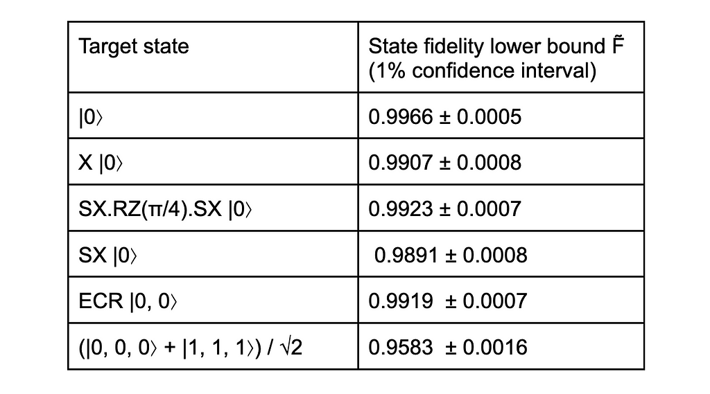
Summary of results and discussion

Let us summarise our results in a table of fidelity lower bounds for the circuits we considered, using IBM QPUs.

We find that the fidelity of states produced by circuits with a minimal number of basis gate is around 99%, which is not a small achievement. As we add more qubits and gates, the fidelity decreases, as we see with the 96% fidelity for the 3-qubit state, whose circuit has 13 basis gates. With more qubits and circuit depth, the fidelity would decrease further, to the point that the quantum computation would be completely unreliable. Nevertheless, these results look quite encouraging for the future of quantum computing.

It is likely that more accurate and rigorous methods exist to evaluate the fidelity of the state produced by a quantum circuit, giving more robust bounds. We are just not aware of them. The main point was to provide hands-on examples of Qiskit circuit manipulations for beginners and to get approximate quantum noise estimates.

While we have run a number of circuits to estimate quantum noise, we have only scratched the surface of the topic. There are many ways to go further, but one important idea to make progress is to make assumptions on the form of the quantum noise, namely to develop a model for a quantum channel representing the action of the noise on a state. This would typically involve a separation between “coherent” noise, preserving the purity of the state, which can be described with a unitary operation, and “incoherent” noise, representing interactions with the environment. The Qiskit Summer School lecture on the topic provides a gentle introduction to these ideas.

Finally, here are a few reviews related to quantum computing, if you want to learn more on this topic. [1] is an introduction to quantum algorithms. [2] is a review of quantum mitigation techniques for near-term quantum devices. [3] is an introduction to quantum error correction theory. [4] is a review of quantum computing ideas and physical realisation of quantum processors in 2022, aimed at a non-scientific audience.

Thanks for getting to the end of this blogpost. I hope you had some fun and learned a thing or two.

Unless otherwise noted, all images are by the author

[1] Blekos, Kostas and Brand, Dean and Ceschini, Andrea and Chou, Chiao-Hui and Li, Rui-Hao and Pandya, Komal and Summer, Alessandro, Quantum Algorithm Implementations for Beginners (2023), Physics Reports Volume 1068, 2 June 2024.

[2] Cai, Zhenyu and Babbush, Ryan and Benjamin, Simon C. and Endo, Suguru and Huggins, William J. and Li, Ying and McClean, Jarrod R. and O’Brien, Thomas E., Quantum error mitigation (2023), Reviews of Modern Physics 95, 045005.

[3] J. Roffe, Quantum error correction: an introductory guide (2019), Contemporary Physics, Oct 2019.

[3] A. K. Fedorov, N. Gisin, S. M. Beloussov and A. I. Lvovsky, Quantum computing at the quantum advantage threshold: a down-to-business review (2022).

---

Measuring Quantum Noise in IBM Quantum Computers was originally published in Towards Data Science on Medium, where people are continuing the conversation by highlighting and responding to this story.