Need extra storage for your new M4 Mac mini but don’t want to pay Apple’s steep upgrade prices? This unique external SSD might be the game-changer you’re looking for
Originally appeared here:
Need extra storage for your new M4 Mac mini but don’t want to pay Apple’s steep upgrade prices? This unique external SSD might be the game-changer you’re looking for
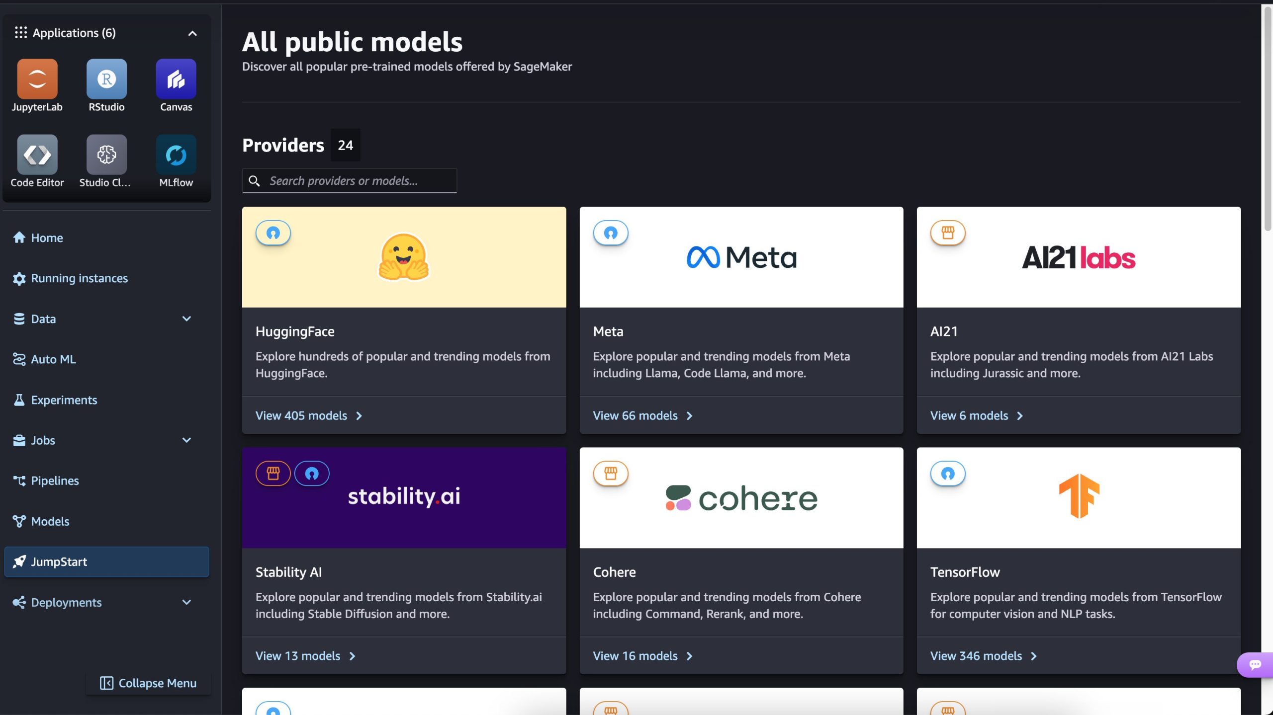
Today, we are excited to announce that Mistral-NeMo-Base-2407 and Mistral-NeMo-Instruct-2407 large language models from Mistral AI that excel at text generation, are available for customers through Amazon SageMaker JumpStart. In this post, we walk through how to discover, deploy and use the Mistral-NeMo-Instruct-2407 and Mistral-NeMo-Base-2407 models for a variety of real-world use cases.
Large Language models are comprised of billions of parameters (weights). For each word it generates, the model has to perform computationally expensive calculations across all of these parameters.
Large Language models accept a sentence, or sequence of tokens, and generate a probability distribution of the next most likely token.
Thus, typically decoding n tokens (or generating n words from the model) requires running the model n number of times. At each iteration, the new token is appended to the input sentence and passed to the model again. This can be costly.
Additionally, decoding strategy can influence the quality of the generated words. Generating tokens in a simple way, by just taking the token with the highest probability in the output distribution, can result in repetitive text. Random sampling from the distribution can result in unintended drift.
Thus, a solid decoding strategy is required to ensure both:
High Quality Outputs
Fast Inference Time
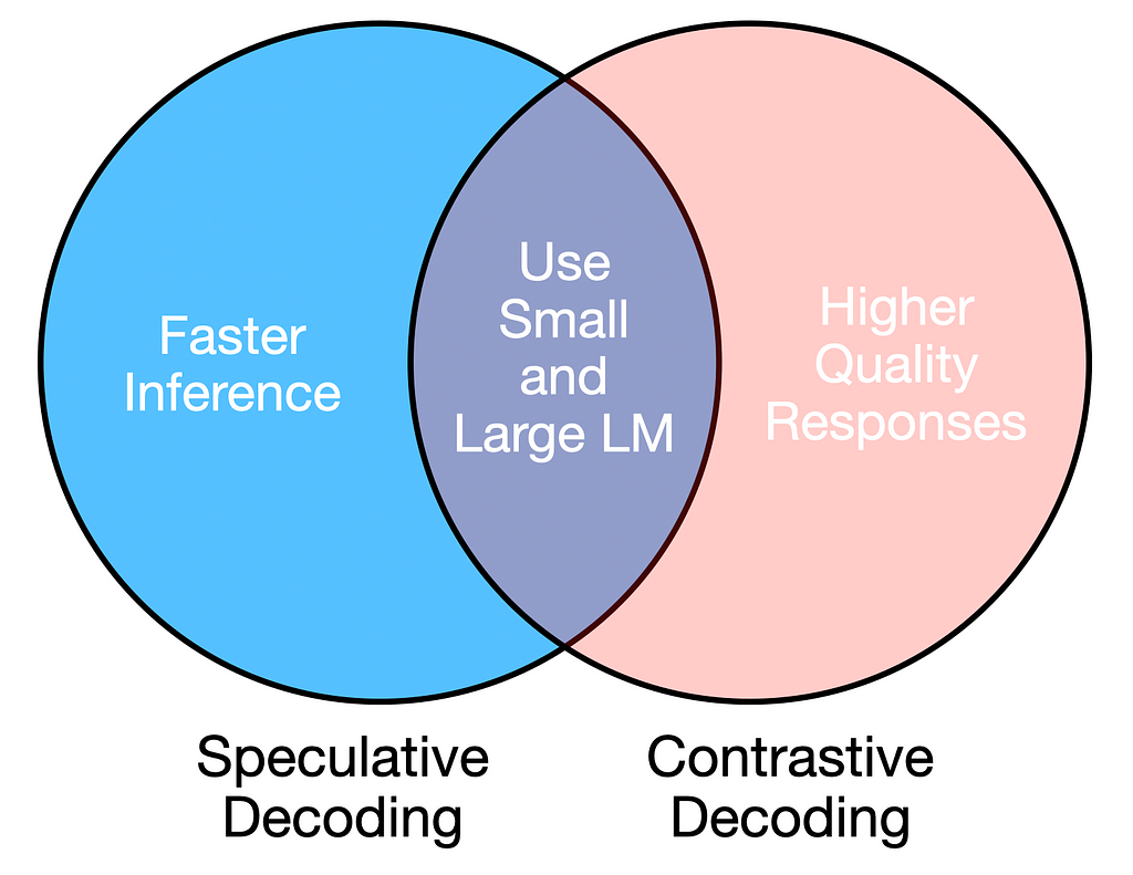
Both requirements can be addressed by using a combination of a large and small language model, as long as the amateur and expert models are similar (e.g., same architecture but different sizes).
Target/Large Model: Main LM with larger number of parameters (e.g. OPT-13B)
Amateur/Small Model: Smaller version of Main LM with fewer parameters (e.g. OPT-125M)
Speculative and contrastive decoding leverage large and small LLMs to achieve reliable and efficient text generation.
Contrastive Decoding for High Quality Inference
Contrastive Decoding is a strategy that exploits the fact that that failures in large LLMs (such as repetition, incoherence) are even more pronounced in small LLMs. Thus, this strategy optimizes for the tokens with the highest probability difference between the small and large model.
For a single prediction, contrastive decoding generates two probability distributions:
q = logit probabilities for amateur model
p = logit probabilities for expert model
The next token is chosen based on the following criteria:
Discard all tokens that do not have sufficiently high probability under the expert model (discard p(x) < alpha * max(p))
From the remaining tokens, select the one the with the largest difference between large model and small model log probabilities, max(p(x) – q(x)).
Implementing Contrastive Decoding
from transformers import AutoTokenizer, AutoModelForCausalLM import torch
# Set an alpha threshold to eliminate less confident tokens in expert alpha = 0.1 candidate_exp_prob = torch.max(expert_logits)
# Mask tokens below threshold for expert model V_head = expert_logits < alpha * candidate_exp_prob
# Select the next token from the log-probabilities difference, ignoring masked values token = torch.argmax(log_probs_diff.masked_fill(V_head, -torch.inf)).unsqueeze(0)
# Append token and accumulate generated text input_ids = torch.cat([input_ids, token.unsqueeze(1)], dim=-1)
Speculative decoding is based on the principle that the smaller model must sample from the same distribution as the larger model. Thus, this strategy aims to accept as many predictions from the smaller model as possible, provided they align with the distribution of the larger model.
The smaller model generates n tokens in sequence, as possible guesses. However, all n sequences are fed into the larger expert model as a single batch, which is faster than sequential generation.
This results in a cache for each model, with n probability distributions in each cache.
q = logit probabilities for amateur model
p = logit probabilities for expert model
Next, the sampled tokens from the amateur model are accepted or rejected based on the following conditions:
If probability of the token is higher in expert distribution (p) than amateur distribution (q), or p(x) > q(x), accept token
If probability of token is lower in expert distribution (p) than amateur distribution (q), or p(x) < q(x), reject token with probability 1 – p(x) / q(x)
If a token is rejected, the next token is sampled from the expert distribution or adjusted distribution. Additionally, the amateur and expert model reset the cache and re-generate n guesses and probability distributions p and q.
Here, the blue signifies accepted tokens, and red/green signify tokens rejected and then sampled from the expert or adjusted distribution.
Implementing Speculative Decoding
from transformers import AutoTokenizer, AutoModelForCausalLM import torch
# Sample a token from the adjusted expert distribution normalized_result = clipped_diff / torch.sum(clipped_diff, dim=0, keepdim=True) next_token = sample_from_distribution(normalized_result) input_ids = torch.cat([input_ids, next_token.unsqueeze(1)], dim=-1) else: # Sample directly from the expert logits for the last accepted token next_token = sample_from_distribution(expert_logits[-1]) input_ids = torch.cat([input_ids, next_token.unsqueeze(1)], dim=-1)
return tokenizer.batch_decode(input_ids)
# Example usage prompt = "Large Language models are" generated_text = speculative_decoding(prompt, n_tokens=3, max_length=25) print(generated_text)
Evaluation
We can evaluate both decoding approaches by comparing them to a naive decoding method, where we randomly pick the next token from the probability distribution.
def sequential_sampling(prompt, max_length=50): """ Perform sequential sampling with the given model. """ # Tokenize the input prompt input_ids = tokenizer(prompt, return_tensors="pt").input_ids
with torch.no_grad(): while input_ids.shape[1] < max_length: # Sample from the model output logits for the last token outputs = expert_lm(input_ids, return_dict=True) logits = outputs.logits[:, -1, :]
To evaluate contrastive decoding, we can use the following metrics for lexical richness.
n-gram Entropy: Measures the unpredictability or diversity of n-grams in the generated text. High entropy indicates more diverse text, while low entropy suggests repetition or predictability.
distinct-n: Measures the proportion of unique n-grams in the generated text. Higher distinct-n values indicate more lexical diversity.
from collections import Counter import math
def ngram_entropy(text, n): """ Compute n-gram entropy for a given text. """ # Tokenize the text tokens = text.split() if len(tokens) < n: return 0.0 # Not enough tokens to form n-grams
# Create n-grams ngrams = [tuple(tokens[i:i + n]) for i in range(len(tokens) - n + 1)]
# Compute entropy entropy = -sum((count / total_ngrams) * math.log2(count / total_ngrams) for count in ngram_counts.values()) return entropy
def distinct_n(text, n): """ Compute distinct-n metric for a given text. """ # Tokenize the text tokens = text.split() if len(tokens) < n: return 0.0 # Not enough tokens to form n-grams
# Create n-grams ngrams = [tuple(tokens[i:i + n]) for i in range(len(tokens) - n + 1)]
# Count unique and total n-grams unique_ngrams = set(ngrams) total_ngrams = len(ngrams)
return len(unique_ngrams) / total_ngrams if total_ngrams > 0 else 0.0
prompts = [ "Large Language models are", "Barack Obama was", "Decoding strategy is important because", "A good recipe for Halloween is", "Stanford is known for" ]
for n in range(1, 4): contrastive_entropy_totals[n - 1] += ngram_entropy(contrastive_generated_text, n)
for n in range(1, 3): contrastive_distinct_totals[n - 1] += distinct_n(contrastive_generated_text, n)
# Compute averages naive_entropy_averages = [total / len(prompts) for total in naive_entropy_totals] naive_distinct_averages = [total / len(prompts) for total in naive_distinct_totals] contrastive_entropy_averages = [total / len(prompts) for total in contrastive_entropy_totals] contrastive_distinct_averages = [total / len(prompts) for total in contrastive_distinct_totals]
# Display results print("Naive Sampling:") for n in range(1, 4): print(f"Average Entropy (n={n}): {naive_entropy_averages[n - 1]}") for n in range(1, 3): print(f"Average Distinct-{n}: {naive_distinct_averages[n - 1]}")
print("nContrastive Decoding:") for n in range(1, 4): print(f"Average Entropy (n={n}): {contrastive_entropy_averages[n - 1]}") for n in range(1, 3): print(f"Average Distinct-{n}: {contrastive_distinct_averages[n - 1]}")
The following results show us that contrastive decoding outperforms naive sampling for these metrics.
Naive Sampling: Average Entropy (n=1): 4.990499826537679 Average Entropy (n=2): 5.174765791328267 Average Entropy (n=3): 5.14373124004409 Average Distinct-1: 0.8949694135740648 Average Distinct-2: 0.9951219512195122
Contrastive Decoding: Average Entropy (n=1): 5.182773920916605 Average Entropy (n=2): 5.3495681172235665 Average Entropy (n=3): 5.313720275712986 Average Distinct-1: 0.9028425204970866 Average Distinct-2: 1.0
To evaluate speculative decoding, we can look at the average runtime for a set of prompts for different n values.
prompts = [ "Large Language models are", "Barack Obama was", "Decoding strategy is important because", "A good recipe for Halloween is", "Stanford is known for" ]
# Loop through n_tokens values for n in n_tokens: avg_time_naive, avg_time_speculative = 0, 0
for prompt in prompts: start_time = time.time() _ = sequential_sampling(prompt, max_length=25) avg_time_naive += (time.time() - start_time)
# Labels and title plt.xlabel('n_tokens', fontsize=12) plt.ylabel('Average Time (s)', fontsize=12) plt.title('Speculative Decoding Runtime vs n_tokens', fontsize=14) plt.legend() plt.grid(axis='y', linestyle='--', alpha=0.7)
# Show the plot plt.show() plt.savefig("plot.png")
We can see that the average runtime for the naive decoding is much higher than for speculative decoding across n values.
Combining large and small language models for decoding strikes a balance between quality and efficiency. While these approaches introduce additional complexity in system design and resource management, their benefits apply to conversational AI, real-time translation, and content creation.
These approaches require careful consideration of deployment constraints. For instance, the additional memory and compute demands of running dual models may limit feasibility on edge devices, though this can be mitigated through techniques like model quantization.
Unless otherwise noted, all images are by the author.
A potential class-action lawsuit alleging that Apple tricked users into having to pay for iCloud is probably now completely dead, having lost an appeal before the Ninth Circuit.
Judges have not said Apple’s 5GB free iCloud space is good or bad, the plaintiffs just haven’t made their case
The case centered on the claim that it is “virtually impossible” for a user’s requirements to be satisfied with the 5GB tier, and that it was effectively impossible for users to reduce their iCloud use. However, as noted by Law360, two of the plaintiffs were reportedly still on the 5GB tier.
Three Ninth Circuit judges considered the appeal, but said the plaintiffs had failed to prove their claims. The judges also noted that users have the option to turn off iCloud if they wish.
Rumors continue to swirl that Apple will launch a new iPhone 17 Slim in 2025. Why does Apple think anyone wants it?
A render of what the iPhone 17 Slim could look like
In a world where people want their devices to last for longer than ever on a single charge, shouldn’t tech companies like Apple focus on bigger, better batteries rather than slimming phones down instead?
The rumors surrounding the iPhone 17 Slim have been around for a little while at this point but the consensus has settled on a couple of notable things. The most is obviously where the name comes from — the fact the iPhone 17 Slim will be thinner than other models on sale alongside it.
Following the introduction of new Mac models in October, Apple has shaken up its desktop Mac roster. Here’s what you should buy this holiday season, at just about any price point.
Apple’s current crop of desktop Macs
Price is an important factor when choosing your next Mac. The more budget that you have available, the better the Mac you can get.
However, while Apple does cover a wide array of price points, it also has multiple choices available for many of them. Add in the number of configurable elements, and it can become a bewildering decision.
The redesign of the M4 Mac mini could’ve been even smaller, Apple executives have admitted, but there were quite a few tradeoffs needed to produce the best version yet.
The M4 Mac mini [middle] between an older Mac mini [below] and an Apple TV [above]
Apple’s revamp of the Mac mini with the M4 and M4 Pro chip led to a much more compact design with quite a few physical changes. Aside from size, it also saw a shift of ports to the front, as well as the under-mounted power button.
In talking about the redesign effort to Fast Company, Apple VP of hardware engineering Kate Bergeron and Mac marketing’s Sophie Le Guen explained that it was a balancing act.
We use cookies on our website to give you the most relevant experience by remembering your preferences and repeat visits. By clicking “Accept”, you consent to the use of ALL the cookies.
This website uses cookies to improve your experience while you navigate through the website. Out of these, the cookies that are categorized as necessary are stored on your browser as they are essential for the working of basic functionalities of the website. We also use third-party cookies that help us analyze and understand how you use this website. These cookies will be stored in your browser only with your consent. You also have the option to opt-out of these cookies. But opting out of some of these cookies may affect your browsing experience.
Necessary cookies are absolutely essential for the website to function properly. These cookies ensure basic functionalities and security features of the website, anonymously.
Cookie
Duration
Description
cookielawinfo-checkbox-analytics
11 months
This cookie is set by GDPR Cookie Consent plugin. The cookie is used to store the user consent for the cookies in the category "Analytics".
cookielawinfo-checkbox-functional
11 months
The cookie is set by GDPR cookie consent to record the user consent for the cookies in the category "Functional".
cookielawinfo-checkbox-necessary
11 months
This cookie is set by GDPR Cookie Consent plugin. The cookies is used to store the user consent for the cookies in the category "Necessary".
cookielawinfo-checkbox-others
11 months
This cookie is set by GDPR Cookie Consent plugin. The cookie is used to store the user consent for the cookies in the category "Other.
cookielawinfo-checkbox-performance
11 months
This cookie is set by GDPR Cookie Consent plugin. The cookie is used to store the user consent for the cookies in the category "Performance".
viewed_cookie_policy
11 months
The cookie is set by the GDPR Cookie Consent plugin and is used to store whether or not user has consented to the use of cookies. It does not store any personal data.
Functional cookies help to perform certain functionalities like sharing the content of the website on social media platforms, collect feedbacks, and other third-party features.
Performance cookies are used to understand and analyze the key performance indexes of the website which helps in delivering a better user experience for the visitors.
Analytical cookies are used to understand how visitors interact with the website. These cookies help provide information on metrics the number of visitors, bounce rate, traffic source, etc.
Advertisement cookies are used to provide visitors with relevant ads and marketing campaigns. These cookies track visitors across websites and collect information to provide customized ads.