
The Moto Edge 50 Pro and Edge 50 Ultra look set to lock horns with the Google Pixel 8 series.
Originally appeared here:
The new Moto Edge 50 series takes on Google Pixel phones with real design flair and solid specs

Originally appeared here:
The new Moto Edge 50 series takes on Google Pixel phones with real design flair and solid specs


Go Here to Read this Fast! When is the next Lego Fortnite update?
Originally appeared here:
When is the next Lego Fortnite update?
Originally appeared here:
Prime Video’s new Outer Range trailer suggests season 2 of the genre-bending sci-fi show will be even stranger
Originally appeared here:
Showing your true feelings in Microsoft Teams is finally getting a lot more inclusive
Originally appeared here:
Broadcom backs down on VMware pricing rules as EU begins investigation following complaints

Go Here to Read this Fast! NYT Connections answers today for April 16
Originally appeared here:
NYT Connections answers today for April 16
Go Here to Read this Fast! Leveraging effective data management for competitive advantage
Originally appeared here:
Leveraging effective data management for competitive advantage


We live in an amazing time of Large Language Models like ChatGPT, GPT-4, and Claude that can perform multiple amazing tasks. In practically every field, ranging from education, healthcare to arts and business, Large Language Models are being used to facilitate efficiency in delivering services. Over the past year, many brilliant open-source Large Language Models, such as Llama, Mistral, Falcon, and Gemma, have been released. These open-source LLMs are available for everyone to use, but deploying them can be very challenging as they can be very slow and require a lot of GPU compute power to run for real-time deployment. Different tools and approaches have been created to simplify the deployment of Large Language Models.
Many deployment tools have been created for serving LLMs with faster inference, such as vLLM, c2translate, TensorRT-LLM, and llama.cpp. Quantization techniques are also used to optimize GPUs for loading very large Language Models. In this article, I will explain how to deploy Large Language Models with vLLM and quantization.
Some of the major factors that affect the speed performance of a Large Language Model are GPU hardware requirements and model size. The larger the size of the model, the more GPU compute power is required to run it. Common benchmark metrics used in measuring the speed performance of a Large Language Model are Latency and Throughput.
Latency: This is the time required for a Large Language Model to generate a response. It is usually measured in seconds or milliseconds.
Throughput: This is the number of tokens generated per second or millisecond from a Large Language Model.
Below are the two required packages for running a Large Language Model: Hugging Face transformers and accelerate.
pip3 install transformers
pip3 install accelerate
Phi-2 is a state-of-the-art foundation model from Microsoft with 2.7 billion parameters. It was pre-trained with a variety of data sources, ranging from code to textbooks. Learn more about Phi-2 from here.
Latency: 2.739394464492798 seconds
Throughput: 32.36171766303386 tokens/second
Generate a python code that accepts a list of numbers and returns the sum. [1, 2, 3, 4, 5]
A: def sum_list(numbers):
    total = 0
    for num in numbers:
        total += num
    return total

print(sum_list([1, 2, 3, 4, 5]))
Step By Step Code Breakdown
Line 6–10: Loaded Phi-2 model and tokenized the prompt “Generate a python code that accepts a list of numbers and returns the sum.”
Line 12- 18: Generated a response from the model and obtained the latency by calculating the time required to generate the response.
Line 21–23: Obtained the total length of tokens in the response generated, divided it by the latency and calculated the throughput.
This model was run on an A1000 (16GB GPU), and it achieves a latency of 2.7 seconds and a throughput of 32 tokens/second.
vLLM is an open source LLM library for serving Large Language Models at low latency and high throughput.
The transformer is the building block of Large Language Models. The transformer network uses a mechanism called the attention mechanism, which is used by the network to study and understand the context of words. The attention mechanism is made up of a bunch of mathematical calculations of matrices known as attention keys and values. The memory used by the interaction of these attention keys and values affects the speed of the model. vLLM introduced a new attention mechanism called PagedAttention that efficiently manages the allocation of memory for the transformer’s attention keys and values during the generation of tokens. The memory efficiency of vLLM has proven very useful in running Large Language Models at low latency and high throughput.
This is a high-level explanation of how vLLM works. To learn more in-depth technical details, visit the vLLM documentation.
vLLM: Easy, Fast, and Cheap LLM Serving with PagedAttention
Install vLLM
pip3 install vllm==0.3.3
Latency: 1.218436622619629seconds
Throughput: 63.15334836428132tokens/second
 [1, 2, 3, 4, 5]
A: def sum_list(numbers):
    total = 0
    for num in numbers:
        total += num
    return total

numbers = [1, 2, 3, 4, 5]
print(sum_list(numbers))
Step By Step Code Breakdown
Line 1–3: Imported required packages from vLLM for running Phi-2.
Line 5–8: Loaded Phi-2 with vLLM, defined the prompt and set important parameters for running the model.
Line 10–16: Generated the model’s response using llm.generate and computed the latency.
Line 19–21: Obtained the length of total tokens generated from the response, divided the length of tokens by the latency to get the throughput.
Line 23–24: Obtained the generated text.
I ran Phi-2 with vLLM on the same prompt, “Generate a python code that accepts a list of numbers and returns the sum.” On the same GPU, an A1000 (16GB GPU), vLLM produces a latency of 1.2 seconds and a throughput of 63 tokens/second, compared to Hugging Face transformers’ latency of 2.85 seconds and a throughput of 32 tokens/second. Running a Large Language Model with vLLM produces the same accurate result as using Hugging Face, with much lower latency and higher throughput.
Note: The metrics (latency and throughput) I obtained for vLLM are estimated benchmarks for vLLM performance. The model generation speed depends on many factors, such as the length of the input prompt and the size of the GPU. According to the official vLLM report, running an LLM model on a powerful GPU like the A100 in a production setting with vLLM achieves 24x higher throughput than Hugging Face Transformers.
The way I calculated the latency and throughput for running Phi-2 is experimental, and I did this to explain how vLLM accelerates a Large Language Model’s performance. In the real-world use case of LLMs, such as a chat-based system where the model outputs a token as it is generated, measuring the latency and throughput is more complex.
A chat-based system is based on streaming output tokens. Some of the major factors that affect the LLM metrics are Time to First Token (the time required for a model to generate the first token), Time Per Output Token (the time spent per output token generated), the input sequence length, the expected output, the total expected output tokens, and the model size. In a chat-based system, the latency is usually a combination of Time to First Token and Time Per Output Token multiplied by the total expected output tokens.
The longer the input sequence length passed into a model, the slower the response. Some of the approaches used in running LLMs in real-time involve batching users’ input requests or prompts to perform inference on the requests concurrently, which helps in improving the throughput. Generally, using a powerful GPU and serving LLMs with efficient tools like vLLM improves both the latency and throughput in real-time.
Run the vLLM deployment on Google Colab
Quantization is the conversion of a machine learning model from a higher precision to a lower precision by shrinking the model’s weights into smaller bits, usually 8-bit or 4-bit. Deployment tools like vLLM are very useful for inference serving of Large Language Models at very low latency and high throughput. We are able to run Phi-2 with Hugging Face and vLLM conveniently on the T4 GPU on Google Colab because it is a smaller LLM with 2.7 billion parameters. For example, a 7-billion-parameter model like Mistral 7B cannot be run on Colab with either Hugging Face or vLLM. Quantization is best for managing GPU hardware requirements for Large Language Models. When GPU availability is limited and we need to run a very large Language Model, quantization is the best approach to load LLMs on constrained devices.
It is a python library built with custom quantization functions for shrinking model’s weights into lower bits(8-bit and 4-bit).
Install BitsandBytes
pip3 install bitsandbytes
Mistral 7B, a 7-billion-parameter model from MistralAI, is one of the best state-of-the-art open-source Large Language Models. I will go through a step-by-step process of running Mistral 7B with different quantization techniques that can be run on the T4 GPU on Google Colab.
Quantization with 8bit Precision: This is the conversion of a machine learning model’s weight into 8-bit precision. BitsandBytes has been integrated with Hugging Face transformers to load a language model using the same Hugging Face code, but with minor modifications for quantization.
Line 1: Imported the needed packages for running model, including the BitsandBytesConfig library.
Line 3–4: Defined the quantization config and set the parameter load_in_8bit to true for loading the model’s weights in 8-bit precision.
Line 7–9: Passed the quantization config into the function for loading the model, set the parameter device_map for bitsandbytes to automatically allocate appropriate GPU memory for loading the model. Finally loaded the tokenizer weights.
Quantization with 4bit Precision: This is the conversion of a machine learning model’s weight into 4-bit precision.
The code for loading Mistral 7B in 4-bit precision is similar to that of 8-bit precision except for a few changes:
NF4 (4-bit Normal Float) from QLoRA is an optimal quantization approach that yields better results than the standard 4-bit quantization. It is integrated with double quantization, where quantization occurs twice; quantized weights from the first stage of quantization are passed into the next stage of quantization, yielding optimal float range values for the model’s weights. According to the report from the QLoRA paper, NF4 with double quantization does not suffer from a drop in accuracy performance. Read more in-depth technical details about NF4 and Double Quantization from the QLoRA paper:
QLoRA: Efficient Finetuning of Quantized LLMs
Line 4–9: Extra parameters were set the BitsandBytesConfig:
Line 11–13: Loaded the model’s weights and tokenizer.
Full Code for Model Quantization
<s> [INST] What is Natural Language Processing? [/INST] Natural Language Processing (NLP) is a subfield of artificial intelligence (AI) and
computer science that deals with the interaction between computers and human language. Its main objective is to read, decipher,
understand, and make sense of the human language in a valuable way. It can be used for various tasks such as speech recognition,
text-to-speech synthesis, sentiment analysis, machine translation, part-of-speech tagging, name entity recognition,
summarization, and question-answering systems. NLP technology allows machines to recognize, understand,
 and respond to human language in a more natural and intuitive way, making interactions more accessible and efficient.</s>
Quantization is a very good approach for optimizing the running of very Large Language Models on smaller GPUs and can be applied to any model, such as Llama 70B, Falcon 40B, and mpt-30b. According to reports from the LLM.int8 paper, very Large Language Models suffer less from accuracy drops when quantized compared to smaller ones. Quantization is best applied to very Large Language Models and does not work well for smaller models because of the loss in accuracy performance.
Run Mixtral 7B Quantization on Google Colab
In this article, I provided a step-by-step approach to measuring the speed performance of a Large Language Model, explained how vLLM works, and how it can be used to improve the latency and throughput of a Large Language Model. Finally, I explained quantization and how it is used to load Large Language Models on small-scale GPUs.
Reach to me via:
Email: [email protected]
Linkedin: https://www.linkedin.com/in/ayoola-olafenwa-003b901a9/
References
Deploying Large Language Models: vLLM and QuantizationStep by Step Guide on How to Accelerate… was originally published in Towards Data Science on Medium, where people are continuing the conversation by highlighting and responding to this story.
Originally appeared here:
Deploying Large Language Models: vLLM and QuantizationStep by Step Guide on How to Accelerate…

In recent years, the Synthetic Control (SC) approach has gained increasing adoption in industry for measuring the the Average Treatment Effect (ATE) of interventions when Randomized Control Trials (RCTs) are not available. One such example is measuring the financial impact of outdoor advertisements on billboards whereby we cannot conduct random treatment assignment in practice.
The basic idea of SC is to estimate ATE by comparing the treatment group against the predicted counterfactual. However, applying SC in practice is usually challenged by the limited knowledge of its validity due to the absence of the true counterfactual in the real world. To mitigate the concern, in this article, I would like to discuss the actionable best practices that help to maximise the reliability of the SC estimation.
The insights and conclusions are obtained through experiments based on diverse synthetic data. The code for data generation, causal inference modeling, and analysis is available in the Jupyter notebook hosted on Github.
The key to measure the ATE of such events is to identify the counterfactual of the treatment group, which is the treatment group in the absence of the treatment, and quantify the post-treatment difference between the two. It is simple for RCTs as the randomised control statistically approximates the counterfactual. However, it’s challenging otherwise due to the unequal pre-experiment statistics between the treatment and control.
As a causal inference technique, SC represents the counterfactual by a synthetic control group created based on some untreated control units. This synthetic control group statistically equals the treatment group pre treatment and is expected to approximate the untreated behaviour of the treatment group post treatment. Mathematically presented below, it is created using the function f whose parameters are obtained by minimising the pre-treatment difference between the treated group and the control synthesised by f [1]:
In practice, the popular options for the function f include but are not limited to the weighted sum [1], Bayesian Structural Time Series (BSTS) [2], etc.
Despite the solid theoretical foundation, applying SC in practice usually faces the challenge that we don’t know how accurate the estimated ATE is because there exists no post-treatment counterfactual in reality to validate the synthesised one. However, there are some actions we can take to optimise the modeling process and maximise the reliability. Next, I will describe these actions and demonstrate how they influence the estimated ATE via a range of experiments based on the synthetic time-series data with diverse temporal characteristics.
Experiment Setup
All the experiments presented in this article are based on synthetic time-series data. These data are generated using the timeseries-generator package that produces time series capturing the real-world factors including GDP, holidays, weekends, and so on.
The data generation aims to simulate the campaign performance of the stores in New Zealand from 01/01/2019 to 31/12/2019. To make the potential conclusions statistically significant, 500 time series are generated to represent the stores. Each time series has the statistically randomised linear trend, white noise, store factor, holiday factor, weekday factor, and seasonality. A random sample of 10 stores are presented below.
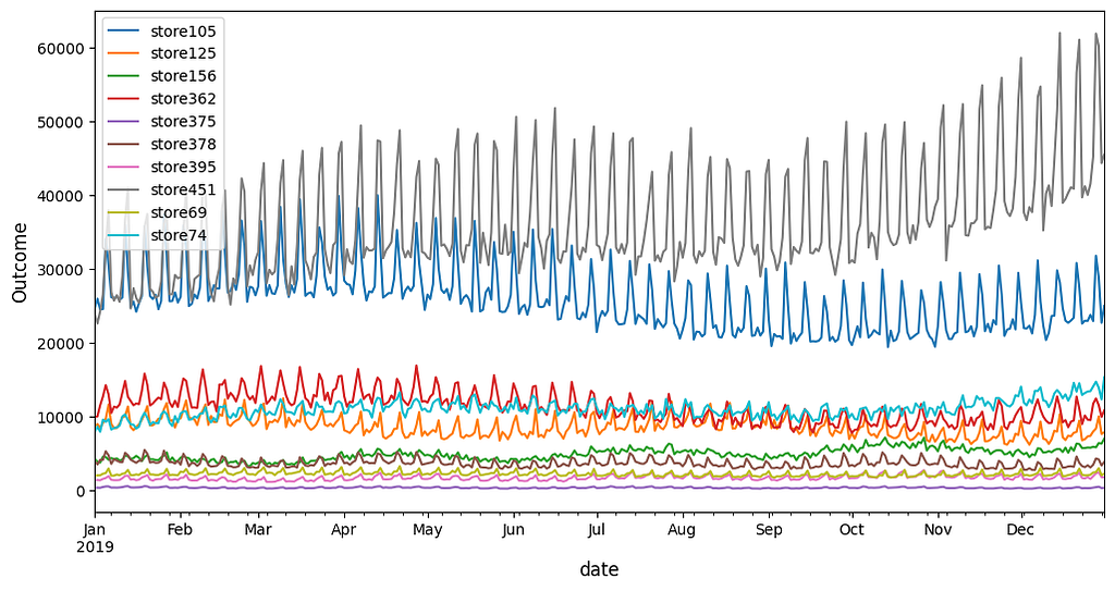
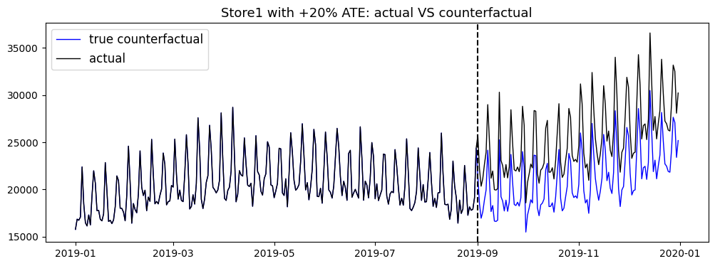
Store1 is selected to be the treatment group whereas others play the role of control groups. Next, the outcome of store1 is uplifted by 20% from 2019-09-01 onwards to simulate the treated behaviour whereas its original outcome serves as the real counterfactual. This 20% uplift establishes the actual ATE to validate the actions later on.
cutoff_date_sc = '2019-09-01'
df_sc.loc[cutoff_date_sc:] = df_sc.loc[cutoff_date_sc:]*1.2
The figure below visualises the simulated treatment effect and the true counterfactual of the treatment group.
Given the synthetic data, the BSTS in Causalimpact is adopted to estimate the synthesised ATE. Then, the estimation is compared against the actual ATE using Mean Absolute Percentage Error (MAPE) to evaluate the corresponding action.
GitHub – jamalsenouci/causalimpact: Python port of CausalImpact R library
Next, let’s go through the actions along with the related experiments to see how to produce reliable ATE estimation.
Treatment-control Correlation
The first action to achieve reliable ATE estimation is selecting the control groups that exhibit high pre-treatment correlations with the treatment group. The rationale is that a highly correlated control is likely to consistently resemble the untreated treatment group over time.
To validate this hypothesis, let’s evaluate the ATE estimation produced using every single control with its full data since 01/01/2019 to understand the impact of correlation. Firstly, the correlation coefficients between the treatment group (store1) and the control groups (store2 to 499) are calculated [3].
def correlation(x, y):
    shortest = min(x.shape[0], y.shape[0])
    return np.corrcoef(x.iloc[:shortest].values, y.iloc[:shortest].values)[0, 1]
As shown in the figure below, the distribution of the correlations range from -0.1 to 0.9, which provides a comprehensive understanding about the impact across various scenarios.

Then, every individual control is used to predict the counterfactual, estimate the ATE, and report the MAPE. In the figure below, the averaged MAPE of ATE with its 95% confidence interval is plotted against the corresponding pre-treatment correlation. Here, the correlation coefficients are rounded to one decimal place to facilitate aggregation and improve the statistical significance in the analysis. Looking at the results, it is obvious that the estimation shows a higher reliability when the control gets more correlated with the treatment group.

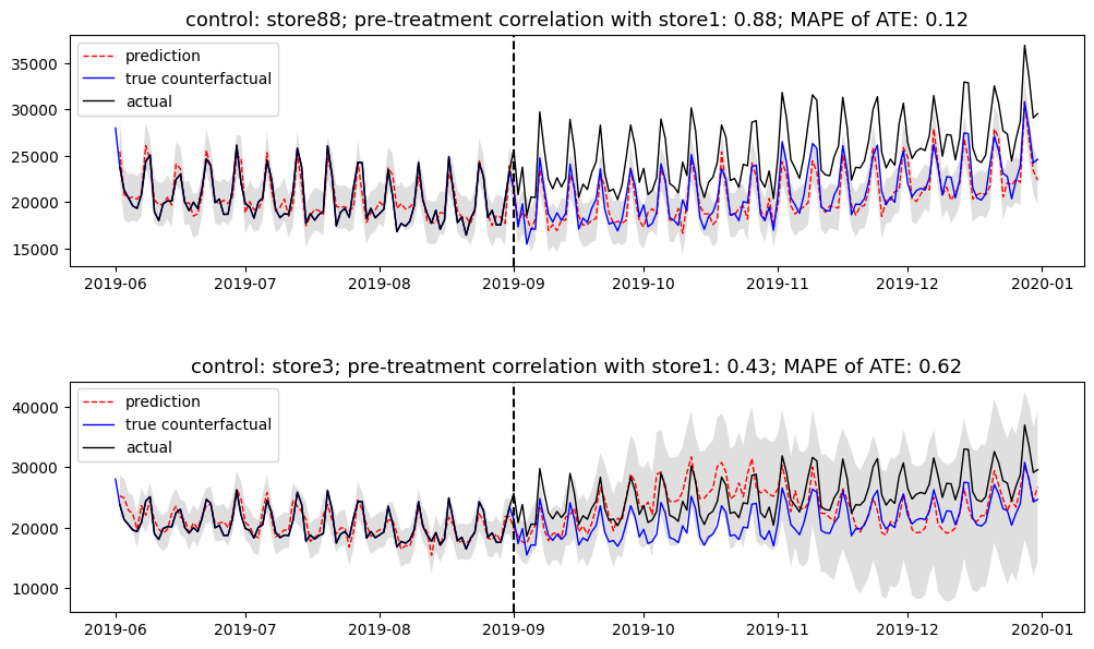
Now let’s see some examples that demonstrate the impact of pre-treatment correlation: store88 with a correlation of 0.88 delivers a MAPE of 0.12 that is superior to 0.62 given by store3 with a correlation of 0.43. Besides the promising accuracy, the probabilistic intervals are correspondingly narrow, which implies high prediction certainty.
Model Fitting Window
Next, the fitting window, which is the length of the pre-treatment interval used for fitting the model, needs to be properly configured. This is because too much context could result in a loss of recency while insufficient context might lead to overfitting.
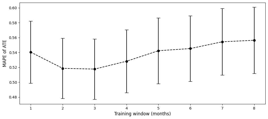
To understand how fitting window impacts the accuracy of ATE estimation, a wide range of values from 1 month to 8 months before the treatment date are experimented. For each fitting window, every single unit of the 499 control groups is evaluated individually and then aggregated to calculate the averaged MAPE with the 95% confidence interval. As depicted in the figure below, there exists a sweet spot nearby 2 and 3 months that optimise the reliability. Identifying the optimal point is outside the scope of this discussion but it’s worth noting that the training window needs to be carefully selected.
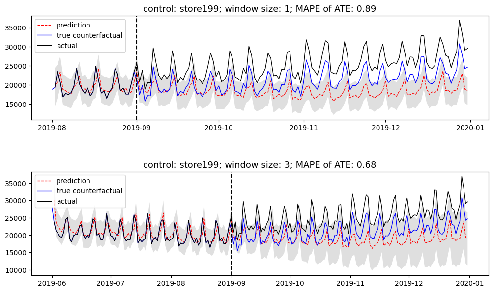
The figure shows two examples: the MAPE of control group 199 is reduced from 0.89 to 0.68 when its fitting window is increased from 1 month to 3 months because the short window contains insufficient knowledge to produce the counterfactual.
Number of Control Units
Lastly, the number of the selected control groups matters.
This hypothesis is validated by investigating the estimation accuracy for different numbers of controls ranging from 1 to 10. In detail, for each control count, the averaged MAPE is calculated based on the estimations produced by 50 random control sets with each containing the corresponding number of control groups. This operation avoids unnecessarily enumerating every possible combination of controls while statistically controls for correlation. In addition, the fitting window is set to 3 months for every estimation.
Looking at the results below, increasing the number of controls is overall leading towards a more reliable ATE estimation.

The examples below demonstrate the effect. The first estimation is generated using store311 whereas the second one further adds store301 and store312.

In this article, I discussed the possible actions that make the SC estimation more reliable. Based on the experiments with diverse synthetic data, the pre-treatment correlation, fitting window, and number of control units are identified as compelling directions to optimise the estimation. Finding the optimal value for each action is out of the scope of this discussion. However, if you feel interested, parameter search using an isolated blank period for validation [4] is one possible solution.
All the images are produced by the author unless otherwise noted. The discussions are inspired by the great work “Synthetic controls in action” [1].
[1] Abadie, Alberto, and Jaume Vives-i-Bastida. “Synthetic controls in action.” arXiv preprint arXiv:2203.06279 (2022).
[2]Brodersen, Kay H., et al. “Inferring causal impact using Bayesian structural time-series models.” (2015): 247–274.
[3]https://medium.com/@dreamferus/how-to-synchronize-time-series-using-cross-correlation-in-python-4c1fd5668c7a
[4]Abadie, Alberto, and Jinglong Zhao. “Synthetic controls for experimental design.” arXiv preprint arXiv:2108.02196 (2021).
Towards Reliable Synthetic Control was originally published in Towards Data Science on Medium, where people are continuing the conversation by highlighting and responding to this story.
Originally appeared here:
Towards Reliable Synthetic Control
Go Here to Read this Fast! Towards Reliable Synthetic Control