Tag: tech

Understanding the power of Lifelong Machine Learning through Q-Learning and Explanation-Based Neural Networks

How does Machine Learning progress from here? Many, if not most, of the greatest innovations in ML have been inspired by Neuroscience. The invention of neural networks and attention-based models serve as prime examples. Similarly, the next revolution in ML will take inspiration from the brain: Lifelong Machine Learning.

Modern ML still lacks humans’ ability to use past information when learning new domains. A reinforcement learning agent who has learned to walk, for example, will learn how to climb from ground zero. Yet, the agent can instead use continual learning: it can apply the knowledge gained from walking to its process of learning to climb, just like how a human would.

Inspired by this property, Lifelong Machine Learning (LLML) uses past knowledge to learn new tasks more efficiently. By approximating continual learning in ML, we can greatly increase the time efficiency of our learners.

To understand the incredible power of LLML, we can start from its origins and build up to modern LLML. In Part 1, we examine Q-Learning and Explanation-Based Neural Networks. In Part 2, we explore the Efficient Lifelong Learning Algorithm and Voyager! I encourage you to read Part 1 before Part 2, though feel free to skip to Part 2 if you prefer!

The Origins of Lifelong Machine Learning

Sebastian Thrun and Tom Mitchell, the fathers of LLML, began their LLML journey by examining reinforcement learning as applied to robots. If the reader has ever seen a visualized reinforcement learner (like this agent learning to play Pokemon), they’ll realize that to achieve any training results in a reasonable human timescale, the agent must be able to iterate through millions of actions (if not much more) over their training period. Robots, though, take multiple seconds to perform each action. As a result, moving typical online reinforcement learning methods to robots results in a significant loss of both the efficiency and capability of the final robot model.

What makes humans so good at real-world learning, where ML in robots is currently failing?

Thrun and Mitchell identified potentially the largest gap in the capabilities of modern ML: its inability to apply past information to new tasks. To solve this issue, they created the first Explanation-Based Neural Network (EBNN), which was the first use of LLML!

To understand how it works, we first can understand how typical reinforcement learning (RL) operates. In RL, our ML model decides the actions of our agent, which we can think of as the ‘body’ that interacts with whatever environment we chose. Our agent exists in environment W with state Z, and when agent takes action A, it receives sensation S (feedback from its environment, for example the position of objects or the temperature). Our environment is a mapping Z x A -> Z (for every action, the environment changes in a specified way). We want to maximize the reward function R: S -> R in our model F: S -> A (in other words we want to choose the action that reaches the best outcome, and our model takes sensation as input and outputs an action). If the agent has multiple tasks to learn, each task has its own reward function, and we want to maximize each function.

We could train each individual task independently. However, Thrun and Michael realized that each task occurs in the same environment with the same possible actions and sensations for our agent (just with different reward functions per task). Thus, they created EBNN to use information from previous problems to solve the current task (LLML)! For example, a robot can use what it’s learned from a cup-flipping task to perform a cup-moving task, since in cup-flipping it has learned how to grab the cup.

To see how EBNN works, we now need to understand the concept of the Q function.

Q* and Q-Learning

Q: S x A -> r is an evaluation function where r represents the expected future total reward after action A in state S. If our model learns an accurate Q, it can simply select the action at any given point that maximizes Q.

Now, our problem reduces to learning an accurate Q, which we call Q*. One such scheme is called Q-Learning, which some think is the inspiration behind OpenAI’s Q* (though the naming might be a complete coincidence).

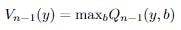
In Q-learning, we define our action policy as function π which outputs an action for each state, and the value of state X as function

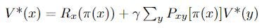
Which we can think of as the immediate reward for action π(x) plus the sum of the probabilities of all possible future actions multiplied by their values (which we compute recursively). We want to find the optimal policy (set of actions) π* such that

(at every state, the policy chooses the action that maximizes V*). As the process repeats Q will become more accurate, improving the agent’s selected actions. Now, we define Q* values as the true expected reward for performing action a:

In Q-learning, we reduce the problem of learning π* to the problem of learning the Q*-values of π*. Clearly, we want to choose the actions with the greatest Q-values.

We divide training into episodes. In the nth episode, we get state x_n, select and perform action a_n, observe y_n, receive reward r_n, and adjust Q values using constant α according to:

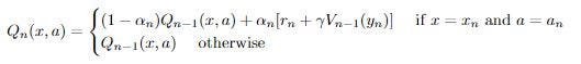
Where

Essentially, we leave all previous Q values the same except for the Q value corresponding to the previous state x and the selected action a. For that Q value, we update it by weighing the previous episode’s Q value by (1 — α) and adding to it our payoff plus the max of the previous episode’s value for the current state y, both weighted by α.

Remember that this algorithm is trying to approximate an accurate Q for each possible action in each possible state. So when we update Q, we update the value for Q corresponding to the old state and the action we took on that episode, since we

The smaller α is, the less we change Q each episode (1 – α will be very large). The larger α is, the less we care about the old value of Q (at α = 1 it is completely irrelevant) and the more we care about what we’ve discovered to be the expected value of our new state.

Let’s consider two cases to gain an intuition for this algorithm and how it updates Q(x, a) after we take action a from state x to reach state y:

1. We go from state x through action a to state y, and are at an ‘end path’ where no more actions are possible. Then, Q(x, a), the expected value for this action and the state before it, should simply be the immediate reward for a (think about why!). Moreover, the higher the reward for a, the more likely we are to choose it in our next episode. Our largest Q value in the previous episode at this state is 0 since no actions are possible, so we are only adding the reward for this action to Q, as intended!
2. Now, our correct Q*s recurse backward from the end! Let’s consider the action b that led from state w to state x, and let’s say we’re now 1 episode later. Now, when we update Q*(w, b), we will add the reward for b to the value for Q*(x, a), since it must be the highest Q value if we chose it before. Thus, our Q(w, b) is now correct as well (think about why)!

Great! Now that you have intuition for Q-learning, we can return to our original goal of understanding:

The Explanation Based Neural Network (EBNN)

We can see that with simple Q-learning, we have no LL property: that previous knowledge is used to learn new tasks. Thrun and Mitchell originated the Explanation Based Neural Network Learning Algorithm, which applies LL to Q-learning! We divide the algorithm into 3 steps.

(1) After performing a sequence of actions, the agent predicts the states that will follow up to a final state s_n, at which no other actions are possible. These predictions will differ from the true observed states since our predictor is currently imperfect (otherwise we’d have finished already)!

(2) The algorithm extracts partial derivatives of the Q function with respect to the observed states. By initially computing the partial derivative of the final reward with respect to the final state s_n, (by the way, we assume the agent is given the reward function R(s)), and we compute slopes backward from the final state using the already computer derivatives using chain rule:

Where M: S x A -> S is our model and R is our final reward.

(3) Now, we’ve estimated the slopes of our Q*s, and we use these in backpropagation to update our Q-values! For those that don’t know, backpropagation is the method through which neural networks learn, where they calculate how the final output of the network changes when each node in the network is changed using this same backward-calculated slope method, and then they adjust the weights and biases of these nodes in the direction that makes the network’s output more desirable (however this is defined by the cost function of the network, which serves the same purpose as our reward function)!

We can think of (1) as the Explaining step (hence the name!), where we look at past actions and try to predict what actions would arise. With (2), we then Analyze these predictions to try to understand how our reward changes with different actions. In (3), we apply this understanding to Learn how to improve our action selection through changing our Qs.

This algorithm increases our efficiency by using the difference between past actions and estimations of past actions as a boost to estimate the efficiency of a certain action path. The next question you might ask is:

How does EBNN help one task’s learning transfer to another?

When we use EBNN applied to multiple tasks, we represent information common between tasks as NN action models, which gives us a boost in learning (a productive bias) through the explanation and analysis process. It uses previously learned, task-independent knowledge when learning new tasks. Our key insight is that we have generalizable knowledge because every task shares the same agent, environment, possible actions, and possible states. The only dependent on each task is our reward function! So by starting from the explanation step with our task-specific reward function, we can use previously discovered states from old tasks as training examples and simply replace the reward function with our current task’s reward function, accelerating the learning process by many fold! The LML fathers discovered a 3 to 4-fold increase in time efficiency for a robot cup-grasping task, and this was only the beginning!

If we repeat this explanation and analysis process, we can replace some of the need for real-world exploration of the agent’s environment required by naive Q-learning! And the more we use it, the more productive it becomes, since (abstractly) there is more knowledge for it to pull from, increasing the likelihood that the knowledge is relevant to the task at hand.

Ever since the fathers of LLML sparked the idea of using task-independent information to learn new tasks, LLML has expanded past not only reinforcement learning in robots but also to the more general ML setting we know today: supervised learning. Paul Ruvolo and Eric Eatons’ Efficient Lifelong Learning Algorithm (ELLA) will get us much closer to understanding the power of LLML!

Please read Part 2: Examining LLML through ELLA and Voyager to see how it works!

Thank you for reading Part 1! Feel free to check out my website anandmaj.com which has my other writing, projects, and art, and follow me on Twitter.

Original Papers and other Sources:

Thrun and Mitchel: Lifelong Robot Learning

Watkins: Q-Learning

Chen and Liu, Lifelong Machine Learning (Inspired me to write this!): https://www.cs.uic.edu/~liub/lifelong-machine-learning-draft.pdf

Unsupervised LL with Curricula: https://par.nsf.gov/servlets/purl/10310051

Deep LL: https://towardsdatascience.com/deep-lifelong-learning-drawing-inspiration-from-the-human-brain-c4518a2f4fb9

Neuro-inspired AI: https://www.cell.com/neuron/pdf/S0896-6273(17)30509-3.pdf

Embodied LL: https://lis.csail.mit.edu/embodied-lifelong-learning-for-decision-making/

EfficientLLA (ELLA): https://www.seas.upenn.edu/~eeaton/papers/Ruvolo2013ELLA.pdf

LL for sentiment classification: https://arxiv.org/abs/1801.02808

Knowledge Basis Idea: https://arxiv.org/ftp/arxiv/papers/1206/1206.6417.pdf

AGI LLLM LLMs: https://towardsdatascience.com/towards-agi-llms-and-foundational-models-roles-in-the-lifelong-learning-revolution-f8e56c17fa66

DEPS: https://arxiv.org/pdf/2302.01560.pdf

Voyager: https://arxiv.org/pdf/2305.16291.pdf

Meta-Learning: https://machine-learning-made-simple.medium.com/meta-learning-why-its-a-big-deal-it-s-future-for-foundation-models-and-how-to-improve-it-c70b8be2931b

Meta Reinforcement Learning Survey: https://arxiv.org/abs/2301.08028

---

The Origins of Lifelong ML: Part 1 of Why LLML is the Next Game-changer of AI was originally published in Towards Data Science on Medium, where people are continuing the conversation by highlighting and responding to this story.

The art of getting quick gains with agile model production

This post was written together with and inspired by Yuval Cohen

Introduction

Every day, numerous data science projects are discarded due to insufficient prediction accuracy. It’s a regrettable outcome, considering that often these models could be exceptionally well-suited for some subsets of the dataset.

Data Scientists often try to improve their models by using more complex models and by throwing more and more data at the problem. But many times there is a much simpler and more productive approach: Instead of trying to make all of our predictions better all at once, we could start by making good predictions for the easy parts of the data, and only then work on the harder parts.

This approach can greatly affect our ability to solve real-world problems. We start with the quick gain on the easy problems and only then focus our effort on the harder problems.

Thinking Agile

Agile production means focusing on the easy data first, and only after it has been properly modelled, moving on the the more complicated tasks. This allows a workflow that is iterative, value-driven, and collaborative.

It allows for quicker results, adaptability to changing circumstances, and continuous improvement, which are core ideas of agile production.

1. Iterative and incremental approach: work in short, iterative cycles. Start by achieving high accuracy for the easy problems and then move on to the harder parts.
2. Focus on delivering value: work on the problem with the highest marginal value for your time.
3. Flexibility and adaptability: Allow yourself to adapt to changing circumstances. For example, a client might need you to focus on a certain subset of the data — once you’ve solved that small problem, the circumstances have changed and you might need to work on something completely different. Breaking the problem into small parts allows you to adapt to the changing circumstances.
4. Feedback and continuous improvement: By breaking up a problem you allow yourself to be in constant and continuous improvement, rather than waiting for big improvements in large chunks.
5. Collaboration: Breaking the problem into small pieces promotes parallelization of the work and collaboration between team members, rather than putting all of the work on one person.

Breaking down the complexity

In real-world datasets, complexity is the rule rather than the exception. Consider a medical diagnosis task, where subtle variations in symptoms can make the difference between life-threatening conditions and minor ailments. Achieving high accuracy in such scenarios can be challenging, if not impossible, due to the inherent noise and nuances in the data.

This is where the idea of coverage comes into play. Coverage refers to the portion of the data that a model successfully predicts or classifies with high confidence or high precision. Instead of striving for high accuracy across the entire dataset, researchers can choose to focus on a subset of the data where prediction is relatively straightforward. By doing so, they can achieve high accuracy on this subset while acknowledging the existence of a more challenging, uncovered portion.

For instance, consider a trained model with a 50% accuracy rate on a test dataset. In this scenario, it’s possible that if we could identify and select only the predictions we are very sure about (although we should decide what “very sure” means), we could end up with a model that covers fewer cases, let’s say around 60%, but with significantly improved accuracy, perhaps reaching 85%.

I don’t know any product manager who would say no in such a situation. Especially if there is no model in production, and this is the first model.

The two-step model

We want to divide our data into two distinct subsets: the covered and the uncovered. The covered data is the part of the data where the initial model achieves high accuracy and confidence. The uncovered data is the part of the data where our model does not give confident predictions and does not achieve high accuracy.

In the first step, a model is trained on the data. Once we identify a subset of data where the model achieves high accuracy, we deploy that model and let it run on that subset — the covered data.

In the second step, we move our focus to the uncovered data. We try to develop a better model for this data by collecting more data, using more advanced algorithms, feature engineering, and incorporating domain-specific knowledge to find patterns in the data.

At this step, the first thing you should do is look at the errors by eye. Many times you will easily identify many patterns this way before using any fancy tricks.

An example

This example will show how the concept of agile workflow can create great value. This is a very simple example that is meant to visualize this concept. Real-life examples will be a lot less obvious but the idea that you will see here is just as relevant.

Let’s look at this two-dimensional data that I simulated from three equally sized classes.

num_samples_A = 500
num_samples_B = 500
num_samples_C = 500


# Class A
mean_A = [3, 2]
cov_A = [[0.1, 0], [0, 0.1]]  # Low variance
class_A = np.random.multivariate_normal(mean_A, cov_A, num_samples_A)

# Class B
mean_B = [0, 0]
cov_B = [[1, 0.5], [0.5, 1]]  # Larger variance with some overlap with class C
class_B = np.random.multivariate_normal(mean_B, cov_B, num_samples_B)

# Class C
mean_C = [0, 1]
cov_C = [[2, 0.5], [0.5, 2]]  # Larger variance with some overlap with class B
class_C = np.random.multivariate_normal(mean_C, cov_C, num_samples_C)

Now we try to fit a machine learning classifier to this data, it looks like an SVM classifier with a Gaussian (‘rbf’) kernel might do the trick:

import pandas as pd
from sklearn.model_selection import train_test_split
from sklearn.linear_model import LogisticRegression
from sklearn.svm import SVC

# Creating DataFrame
data = np.concatenate([class_A, class_B, class_C])
labels = np.concatenate([np.zeros(num_samples_A), np.ones(num_samples_B), np.ones(num_samples_C) * 2])
df = pd.DataFrame(data, columns=['x', 'y'])
df['label'] = labels.astype(int)

# Splitting data into train and test sets
X_train, X_test, y_train, y_test = train_test_split(df[['x', 'y']], df['label'], test_size=0.2, random_state=42)

# Training SVM model with RBF kernel
svm_rbf = SVC(kernel='rbf', probability= True)
svm_rbf.fit(X_train, y_train)

# Predict probabilities for each class
svm_rbf_probs = svm_rbf.predict_proba(X_test)

# Get predicted classes and corresponding confidences
svm_rbf_predictions = [(X_test.iloc[i]['x'], X_test.iloc[i]['y'], true_class, np.argmax(probs), np.max(probs)) for i, (true_class, probs) in enumerate(zip(y_test, svm_rbf_probs))]

svm_predictions_df = pd.DataFrame(svm_rbf_predictions).rename(columns={0:'x',1:'y' ,2: 'true_class', 3: 'predicted_class', 4: 'confidence'})

How does this model perform on our data?

accuracy = (svm_predictions_df['true_class'] == svm_predictions_df['predicted_class']).mean()*100
print(f'Accuracy = {round(accuracy,2)}%')

Accuracy = 75.33%

75% percent accuracy is disappointing, but does this mean that this model is useless?

Now we want to look at the most confident predictions and see how the model performs on them. How do we define the most confident predictions? We can try out different confidence (predict_proba) thresholds and see what coverage and accuracy we get for each threshold and then decide which threshold meets our business needs.

thresholds = [.5, .55, .6, .65, .7, .75, .8, .85, .9]
results = []

for threshold in thresholds:
    svm_df_covered = svm_predictions_df.loc[svm_predictions_df['confidence'] > threshold]
    coverage = len(svm_df_covered) / len(svm_predictions_df) * 100
    accuracy_covered = (svm_df_covered['true_class'] == svm_df_covered['predicted_class']).mean() * 100

    results.append({'Threshold': threshold, 'Coverage (%)': round(coverage,2), 'Accuracy on covered data (%)': round(accuracy_covered,2)})

results_df = pd.DataFrame(results)
print(results_df)

And we get

Or if we want a more detailed look we can create a plot of the coverage and accuracy by threshold:

We can now select the threshold that fits our business logic. For example, if our company’s policy is to guarantee at least 90% accuracy, then we can choose a threshold of 0.75 and get an accuracy of 90% for 62% of the data. This is a huge improvement to throwing out the model, especially if we don’t have any model in production!

Now that our model is happily working in production on 60% of the data, we can shift our focus to the rest of the data. We can collect more data, do more feature engineering, try more complex models, or get help from a domain expert.

Balancing act

The two-step model allows us to aim for accuracy while acknowledging that it is perfectly fine to start with a high accuracy for only a subset of the data. It is counterproductive to insist that a model will have high accuracy on all the data before deploying it to production.

The agile approach presented in this post aims for resource allocation and efficiency. Instead of spending computational resources on getting high accuracy all across. Focus your resources on where the marginal gain is highest.

Conclusion

In data science, we try to achieve high accuracy. However, in the reality of messy data, we need to find a clever approach to utilize our resources in the best way. Agile model production teaches us to focus on the parts of the data where our model works best, deploy the model for those subsets, and only then start working on a new model for the more complicated part. This strategy will help you make the best use of your resources in the face of real data science problems.

Think production, Think Agile.

---

Coverage vs. Accuracy: Striking a Balance in Data Science was originally published in Towards Data Science on Medium, where people are continuing the conversation by highlighting and responding to this story.

In this post, we explore the performance benefits of Amazon SageMaker (including SMP and SMDDP), and how you can use the library to train large models efficiently on SageMaker. We demonstrate the performance of SageMaker with benchmarks on ml.p4d.24xlarge clusters up to 128 instances, and FSDP mixed precision with bfloat16 for the Llama 2 model.

Amazon Lex is a fully managed artificial intelligence (AI) service with advanced natural language models to design, build, test, and deploy conversational interfaces in applications. It employs advanced deep learning technologies to understand user input, enabling developers to create chatbots, virtual assistants, and other applications that can interact with users in natural language. Managing your […]

Generative artificial intelligence (AI) is transforming the customer experience in industries across the globe. Customers are building generative AI applications using large language models (LLMs) and other foundation models (FMs), which enhance customer experiences, transform operations, improve employee productivity, and create new revenue channels. The biggest concern we hear from customers as they explore the advantages of generative AI is how to protect their highly sensitive data and investments. At AWS, our top priority is safeguarding the security and confidentiality of our customers’ workloads. We think about security across the three layers of our generative AI stack …