Connections is the new puzzle game from the New York Times, and it can be quite difficult. If you need a hand with solving today’s puzzle, we’re here to help.
The NYT Mini crossword might be a lot smaller than a normal crossword, but it isn’t easy. If you’re stuck with today’s crossword, we’ve got answers for you here.
Take-Two Interactive plans to lay off 5 percent of its workforce, or about 600 employees, by the end of the year, as reported in an SEC filing Tuesday. The studio is also canceling several in-development projects. These moves are expected to cost $160 million to $200 million to implement, and should result in $165 million in annual savings for Take-Two.
As the owner of Grand Theft Auto and the parent company of Rockstar Games, 2K, Private Division, Zynga and Gearbox, Take-Two is a juggernaut in the video game industry. It reported $5.3 billion in revenue in 2023, a nearly $2 billion increase over the previous year. Just a few weeks ago, Take-Two agreed to purchase Gearbox, the studio responsible for Borderlands, for $460 million. The company is preparing to release Grand Theft Auto VI in 2025, a move that should bring in billions on its own.
Take-Two instituted a round of layoffs in 2023 across Private Division — the indie label behind Kerbal Space Program, The Outer Worlds and Rollerdrome — and other in-house studios.
An estimated 8,800 people in the video game industry have lost their jobs in 2024 so far, and a total of 10,500 industry employees were laid off in 2023. These are, depressingly, record–breaking figures. Sony laid off about 900 people at PlayStation in February; Microsoft fired about 1,900 workers across its gaming division in January; Riot Games let go more than 500 people that same month — and these are just some of the most recent AAA layoffs. Take-Two is now at the head of this list.
Take-Two executives have been hinting at a “significant cost reduction program” coming this year, but before today, they deflected questions about mass layoffs. In March, CEO Strauss Zelnick said on an investor call, “The hardest thing to do is to lay off colleagues and we have no current plans.”
This article originally appeared on Engadget at https://www.engadget.com/take-two-plans-to-lay-off-5-percent-of-its-employees-by-the-end-of-2024-235903990.html?src=rss
Dive into AlexNet, the first modern CNN, understand its mathematics, implement it from scratch, and explore its applications.
Image generated by DALL-E
Convolutional Neural Networks (CNNs) are a specialized kind of deep neural networks designed primarily for processing structured array data such as images. CNNs operate by recognizing patterns directly from pixel data of images, eliminating the need for manual feature extraction. They are particularly powerful in understanding the spatial hierarchy in images, utilizing learnable filters that process data in patches and thus preserving the spatial relationships between pixels.
These networks are incredibly effective at tasks that involve large amounts of visual data and are widely used in applications ranging from image and video recognition to real-time object detection, playing pivotal roles in advancements like facial recognition technology and autonomous vehicles.
In this article, we’ll explore AlexNet, a groundbreaking CNN architecture that has significantly influenced the field of computer vision. Known for its robust performance on various visual recognition tasks, AlexNet utilizes deep learning to interpret complex imagery directly. We’ll break down the mathematics behind its operations and the coding framework that powers it.
AlexNet is a pioneering deep learning network that rose to prominence after winning the ImageNet Large Scale Visual Recognition Challenge in 2012. Developed by Alex Krizhevsky, Ilya Sutskever, and Geoffrey Hinton, AlexNet significantly lowered the top-5 error rate to 15.3% from the previous best of 26.2%, setting a new benchmark for the field. This achievement highlighted the effectiveness of CNNs that use ReLU activations, GPU acceleration, and dropout regularization to manage complex image classification tasks across large datasets.
The model comprises several layers that have become standard in most deep-learning CNNs today. These include convolutional layers, max-pooling, dropout, fully connected layers, and a softmax output layer. The model’s success demonstrated the practicality of deeper network architectures through creative approaches to design and training.
In this article, we will break down the sophisticated design and mathematical principles that underpin AlexNet. We’ll also review AlexNet’s training procedures and optimization techniques, and we will build it from scratch using PyTorch.
2: Overview of AlexNet Architecture
AlexNet Architecture — Image by Author
2.1: General Layer Structure
AlexNet’s architecture cleverly extracts features through a hierarchical layering system where each layer builds on the previous layers’ outputs to refine the feature extraction process. Here’s a detailed breakdown of its layers and functions:
Input Image The model processes input images resized to 227×227 pixels. Each image has three channels (Red, Green, and Blue), reflecting standard RGB encoding.
Layer Configuration It consists of eight primary layers that learn weights, five of which are convolutional, and the remaining three are fully connected. Between these layers, activation functions, normalization, pooling, and dropout are strategically applied to improve learning efficacy and combat overfitting.
Convolutional Layers The initial layer uses 96 kernels (filters) sized 11x11x3, which convolve with the input image using a stride of 4 pixels. This large stride size helps reduce the output spatial volume size significantly, making the network computationally efficient right from the first layer.
Outputs from the first layer undergo normalization and max-pooling before reaching the second convolutional layer, which consists of 256 kernels each of size 5x5x48. The use of 48 feature maps each corresponds to separate filtered outputs from the previous layer, allowing this layer to mix features effectively.
The third convolutional layer does not follow with pooling or normalization, which typically helps to maintain the feature map’s richness derived from previous layers. It includes 384 kernels of size 3x3x256, directly connected to the outputs of the second layer, enhancing the network’s ability to capture complex features.
The fourth convolutional layer mirrors the third layer’s configuration but uses 384 kernels of size 3x3x192, enhancing the depth of the network without altering the layer’s spatial dimensions.
The final convolutional layer employs 256 kernels of size 3x3x192 and is followed by a max-pooling layer, which helps to reduce dimensionality and provides rotational and positional invariance to the features being learned.
Fully Connected Layers The first fully connected layer is a dense layer with 4096 neurons. It takes the flattened output from the preceding convolutional layers (transformed into a 1D vector) and projects it onto a high-dimensional space to learn non-linear combinations of the features.
The second fully connected layer also features 4096 neurons and includes dropout regularization. Dropout helps prevent overfitting by randomly setting a fraction of input units to zero during training, which encourages the network to learn more robust features that are not reliant on any small set of neurons.
The final fully connected layer comprises 1000 neurons, each corresponding to a class of the ImageNet challenge. This layer is essential for class prediction, and it typically utilizes a softmax function to derive the classification probabilities.
2.2: Output Layer and Softmax Classification
The final layer in AlexNet is a softmax regression layer which outputs a distribution over the 1000 class labels by applying the softmax function to the logits of the third fully connected layer.
The softmax function is given by:
Softmax Function — Image by Author
where zi are the logits or the raw prediction scores for each class from the final fully connected layer.
This layer essentially converts the scores into probabilities by comparing the exponentiated score of each class with the sum of exponentiated scores for all classes, highlighting the most probable class.
The softmax layer not only outputs these probabilities but also forms the basis for the cross-entropy loss during training, which measures the difference between the predicted probability distribution and the actual distribution (the true labels).
3: In-depth Analysis of AlexNet Components
3.1: ReLU Nonlinearity
The Rectified Linear Unit (ReLU) has become a standard activation function for deep neural networks, especially CNNs like AlexNet. Its simplicity allows models to train faster and converge more effectively compared to networks using sigmoid or tanh functions.
The mathematical representation of ReLU is straightforward:
ReLU Function — Image by Author
This function outputs x if x is positive; otherwise, it outputs zero.
ReLU Plot — Image by Author
Graphically, it looks like a ramp function that increases linearly for all positive inputs and is zero for negative inputs.
Advantages Of Sigmoid Over Tanh ReLU has several advantages over traditional activation functions such as sigmoid:
Sigmoid Function — Image by Author
and hyperbolic tangent:
Tanh Function — Image by Author
ReLU helps neural networks converge faster by addressing the vanishing gradient problem. This problem occurs with sigmoid and tanh functions where gradients become very small (approach zero) as inputs become large, in either positive or negative direction. This small gradient slows down the training significantly as it provides very little update to the weights during backpropagation. In contrast, the gradient of the ReLU function is either 0 (for negative inputs) or 1 (for positive inputs), which simplifies and speeds up gradient descent.
It promotes sparsity of the activation. Since it outputs zero for half of its input domain, it inherently produces sparse data representations. Sparse representations seem to be more beneficial than dense representations (as typically produced by sigmoid or tanh functions), particularly in large-scale image recognition tasks where the inherent data dimensionality is very high but the informative part is relatively low.
Moreover, ReLU involves simpler mathematical operations. For any input value, this activation function requires a single max operation, whereas sigmoid and tanh involve more complex exponential functions, which are computationally more expensive. This simplicity of ReLU leads to much faster computational performance, especially beneficial when training deep neural networks on large datasets.
Because the negative part of ReLU’s function is zeroed out, it avoids the problem of outputs that do not change in a non-linear fashion as seen with sigmoid or tanh functions. This characteristic allows the network to model the data more cleanly and avoid potential pitfalls in training dynamics.
AlexNet was one of the pioneering convolutional neural networks to leverage parallel GPU training, managing its deep and computation-heavy architecture. The network operates on two GPUs simultaneously, a core part of its design that greatly improves its performance and practicality.
Layer-wise Distribution AlexNet’s layers are distributed between two GPUs. Each GPU processes half of the neuron activations (kernels) in the convolutional layers. Specifically, the kernels in the third layer receive inputs from all kernel maps of the second layer, whereas the fourth and fifth layers only receive inputs from kernel maps located on the same GPU.
Communication Across GPUs The GPUs need to communicate at specific layers crucial for combining their outputs for further processing. This inter-GPU communication is essential for integrating the results of parallel computations.
Selective Connectivity Not every layer in AlexNet is connected across both GPUs. This selective connectivity reduces the amount of data transferred between GPUs, cutting down on communication overhead and enhancing computation efficiency.
This strategy of dividing not just the dataset but also the network model across two GPUs enables AlexNet to handle more parameters and larger input sizes than if it were running on a single GPU. The extra processing power allows AlexNet to handle its 60 million parameters and the extensive computations required for training deep networks on large-scale image classification tasks efficiently.
Training with larger batch sizes is more feasible with multiple GPUs. Larger batches provide more stable gradient estimates during training, which is vital for efficiently training deep networks. While not directly a result of using multiple GPUs, the ability to train with larger batch sizes and more rapid iteration times helps combat overfitting. The network experiences a more diverse set of data in a shorter amount of time, which enhances its ability to generalize from the training data to unseen data.
3.3: Local Response Normalization
Local Response Normalization (LRN) in AlexNet is a normalization strategy that plays a crucial role in the network’s ability to perform well in image classification tasks. This technique is applied to the output of the ReLU non-linearity activation function.
LRN aims to encourage lateral inhibition, a biological process where activated neurons suppress the activity of neighboring neurons in the same layer. This mechanism works under the “winner-takes-all” principle, where neurons showing relatively high activity suppress the less active neurons around them. This dynamic allows the most significant features relative to their local neighborhood to be enhanced while suppressing the lesser ones.
The LRN layer computes a normalized output for each neuron by performing a sort of lateral inhibition by damping the responses of neurons when their locally adjacent neurons exhibit high activity.
Given a neuron’s activity ax, yi at position (x, y) in the feature map i, the response-normalized activity bx, yi is given by:
Local Response Normalization Formula — Image by Author
where:
ax, yi is the activity of a neuron computed by applying kernel i at position (x, y) and then applying the ReLU function.
N is the total number of kernels in the layer.
The sum runs over n neighboring kernel maps at the same spatial position, and N is the total number of kernels.
k, α, β are hyperparameters whose values are predetermined (in AlexNet, typically n=5, k=2, α=10e−4, β=0.75).
bx, yi is the normalized response of the neuron.
Local Response Normalization (LRN) serves to implement a form of local inhibition among adjacent neurons, which is inspired by the concept of lateral inhibition found in biological neurons. This inhibition plays a vital role in several key areas:
Activity Regulation LRN prevents any single feature map from overwhelming the response of the network by penalizing larger activations that lack support from their surroundings. This squaring and summing of neighboring activations ensures no single feature disproportionately influences the output, enhancing the model’s ability to generalize across various inputs.
Contrast Normalization By emphasizing patterns that stand out relative to their neighbors, LRN functions similarly to contrast normalization in visual processing. This feature highlights critical local features in an image more effectively, aiding in the visual differentiation process.
Error Rate Reduction Incorporating LRN in AlexNet has helped reduce the top-1 and top-5 error rates in the ImageNet classification tasks. It manages the high activity levels of neurons, thereby improving the overall robustness of the network.
3.4: Overlapping Pooling
Overlapping pooling is a technique used in convolutional neural networks (CNNs) to reduce the spatial dimensions of the input data, simplify the computations, and help control overfitting. It modifies the standard non-overlapping (traditional) max-pooling by allowing the pooling windows to overlap.
Traditional Max Pooling In traditional max pooling, the input image or feature map is divided into distinct, non-overlapping regions, each corresponding to the size of the pooling filter, often 2×2. For each of these regions, the maximum pixel value is determined and output to the next layer. This process reduces the data dimensions by selecting the most prominent features from non-overlapping neighborhoods.
For example, assuming a pooling size (z) of 2×2 and a stride (s) of 2 pixels, the filter moves 2 pixels across and 2 pixels down the input field. The stride of 2 ensures there is no overlap between the regions processed by the filter.
Overlapping Pooling in AlexNet Overlapping pooling, used by AlexNet, involves setting the stride smaller than the pool size. This approach allows the pooling regions to overlap, meaning the same pixel may be included in multiple pooling operations. It increases the density of the feature mapping and helps retain more information through the layers.
For example, using a pooling size of 3×3 and a stride of 2 pixels. This configuration means that while the pooling filter is larger (3×3), it moves by only 2 pixels each time it slides over the image or feature map. As a result, adjacent pooling regions share a column or row of pixels that gets processed multiple times, enhancing feature integration.
3.5: Fully Connected Layers and Dropout
In the architecture of AlexNet, after several stages of convolutional and pooling layers, the high-level reasoning in the network is done by fully connected layers. Fully connected layers play a crucial role in transitioning from the extraction of feature maps in the convolutional layers to the final classification.
A fully connected (FC) layer takes all neurons in the previous layer (whether they are the output of another fully connected layer, or a flattened output from a pooling or convolutional layer) and connects each of these neurons to every neuron it contains. In AlexNet, there are three fully connected layers following the convolutional and pooling layers.
The first two fully connected layers in AlexNet have 4096 neurons each. These layers are instrumental in integrating the localized, filtered features that the prior layers have identified into global, high-level patterns that can represent complex dependencies in the inputs. The final fully connected layer effectively acts as a classifier: with one neuron for each class label (1000 for ImageNet), it outputs the network’s prediction for the input image’s category.
Each neuron in these layers applies a ReLU (Rectified Linear Unit) activation function except for the output layer, which uses a softmax function to map the output logits (the raw prediction scores for each class) to a probabilistic distribution over the classes.
The output from the final pooling or convolutional layer typically undergoes flattening before being fed into the fully connected layers. This process transforms the 2D feature maps into 1D feature vectors, making them suitable for processing via traditional neural network techniques. The final layer’s softmax function then classifies the input image by assigning probabilities to each class label based on the feature combinations learned through the network.
3.6: Dropout
Dropout is a regularization technique used to prevent overfitting in neural networks, particularly effective in large networks like AlexNet. Overfitting occurs when a model learns patterns specific to the training data, but which do not generalize to new data.
In AlexNet, dropout is applied to the outputs of the first two fully connected layers. Each neuron in these layers has a probability p (commonly set to 0.5, i.e., 50%) of being “dropped,” meaning it is temporarily removed from the network along with all its incoming and outgoing connections.
If you want to dive deep into Dropout’s math and code, I highly recommend you take a look at section 3.4 of my previous article:
In AlexNet, Stochastic Gradient Descent (SGD) is employed to optimize the network during training. This method updates the network’s weights based on the error gradient of the loss function, where the effective tuning of parameters such as batch size, momentum, and weight decay is critical for the model’s performance and convergence. In today’s article, we will use a Pytorch implementation of SGD, and we will cover a high-level view of this popular optimization technique. If you are interested in a low-level view, scraping its math, and building the optimizer from scratch, take a look at this article:
Let’s cover now the main components of SGD and the settings used in AlexNet:
Batch Size The batch size, which is the number of training examples used to calculate the loss function’s gradient for one update of the model’s weights, is set to 128 in AlexNet. This size strikes a balance between computational efficiency — since larger batches require more memory and computation — and the accuracy of error estimates, which benefit from averaging across more examples.
The choice of a batch size of 128 helps stabilize the gradient estimates, making the updates smoother and more reliable. While larger batches provide a clearer signal for each update by reducing noise in the gradient calculations, they also require more computational resources and may sometimes generalize less effectively from training data to new situations.
Momentum Momentum in SGD helps accelerate the updates in the correct direction and smoothens the path taken by the optimizer. It modifies the update rule by incorporating a fraction of the previous update vector. In AlexNet, the momentum value is 0.9, implying that 90% of the previous update vector contributes to the current update. This high level of momentum speeds up convergence towards the loss function’s minimum, which is particularly useful when dealing with small but consistent gradients.
Using momentum ensures that updates not only move in the right direction but also build up speed along surfaces of the loss function’s topology that have consistent gradients. This aspect is crucial for escaping from any potential shallow local minima or saddle points more effectively.
Weight Decay Weight decay acts as a regularization term that penalizes large weights by adding a portion of the weight values to the loss function. AlexNet sets this parameter at 0.0005 to keep the weights from becoming too large, which could lead to overfitting given the network’s large number of parameters.
Weight decay is essential in complex models like AlexNet, which are prone to overfitting due to their high capacity. By penalizing the magnitude of the weights, weight decay ensures that the model does not rely too heavily on a small number of high-weight features, promoting a more generalized model.
The update rule for AlexNet’s weights can be described as follows:
AlexNet Update Formula — Image by Author
Here:
vt is the momentum-enhanced update vector from the previous step.
μ (0.9 for AlexNet) is the momentum factor, enhancing the influence of the previous update.
ϵ is the learning rate, determining the size of the update steps.
∇L represents the gradient of the loss function for the weights.
λ (0.0005 for AlexNet) is the weight decay factor, mitigating the risk of overfitting by penalizing large weights.
w denotes the weights themselves.
These settings help ensure that the network not only learns efficiently but also achieves robust performance on both seen and unseen data, optimizing the speed and accuracy of training while maintaining the ability to generalize well.
4.2: Initialization
Proper initialization of weights and biases and the careful adjustment of the learning rate are critical to training deep neural networks. These factors influence the rate at which the network converges and its overall performance on both training and validation datasets.
Weights Initialization
In AlexNet, the weights for the convolutional layers are initialized from a zero-mean Gaussian distribution with a standard deviation of 0.01. This narrow standard deviation prevents any single neuron from initially overwhelming the output, ensuring a uniform scale of weight initialization.
Similarly, weights in the fully connected layers are initialized from a Gaussian distribution. Special attention is given to the variance of this distribution to keep the output variance consistent across layers, which is crucial for maintaining the stability of deeper networks.
To get a better understanding of this process let’s build the initialization for AlexNet from scratch in Python:
import numpy as np
def initialize_weights(layer_shapes): weights = [] for shape in layer_shapes: if len(shape) == 4: # This is a conv layer: (out_channels, in_channels, filter_height, filter_width) std_dev = 0.01 # Standard deviation for conv layers fan_in = np.prod(shape[1:]) # product of in_channels, filter_height, filter_width elif len(shape) == 2: # This is a fully connected layer: (out_features, in_features) # He initialization: std_dev = sqrt(2. / fan_in) fan_in = shape[1] # number of input features std_dev = np.sqrt(2. / fan_in) # Recommended to maintain variance for ReLU else: raise ValueError("Invalid layer shape: must be 4D (conv) or 2D (fc)")
initialized_weights = initialize_weights(layer_shapes) for idx, weight in enumerate(initialized_weights): print(f"Layer {idx+1} weights shape: {weight.shape} mean: {np.mean(weight):.5f} std dev: {np.std(weight):.5f}")
The initialize_weights function takes a list of tuples describing the dimensions of each layer’s weights. Convolutional layers expect four dimensions (number of filters, input channels, filter height, filter width), while fully connected layers expect two dimensions (output features, input features).
In the convolutional layers standard deviation is fixed at 0.01, aligned with the original AlexNet configuration to prevent overwhelming outputs by any single neuron.
Fully connected layers use He initialization (good practice for layers using ReLU activation) where the standard deviation is adjusted to sqrt(2/fan_in) to keep the output variance consistent, promoting stable learning in deep networks.
For each layer defined in layer_shapes, weights are initialized from a Gaussian (normal) distribution centered at zero with a calculated
Biases Initialization Biases in some convolutional layers are set to 1, particularly in layers followed by ReLU activations. This initialization pushes the neuron outputs into the positive range of the ReLU function, ensuring they are active from the beginning of training. Biases in other layers are initialized at 0 to start from a neutral output.
Like in certain convolutional layers, biases in fully connected layers are also set to 1. This strategy helps to prevent dead neurons at the start of training by ensuring that neurons are initially in the positive phase of activation.
4.3: Strategy for Adjusting the Learning Rate
AlexNet begins with an initial learning rate of 0.01. This rate is high enough to allow significant updates to the weights, facilitating rapid initial progress without being so high as to risk the divergence of the learning process.
The learning rate is decreased by a factor of 10 at predetermined points during the training. This approach is known as “step decay.” In AlexNet, these adjustments typically occur when the validation error rate stops decreasing significantly. Reducing the learning rate at these points helps refine the weight adjustments, promoting better convergence.
Starting with a higher learning rate helps the model overcome potential local minima more effectively. As the network begins to stabilize, reducing the learning rate helps it settle into broad, flat minima that are generally better for generalization to new data.
As training progresses, lowering the learning rate allows for finer weight adjustments. This gradual refinement helps the model to not only fit the training data better but also improves its performance on validation data, ensuring the model is not just memorizing the training examples but genuinely learning to generalize from them.
5: Building AlexNet in Python
In this section, we detail the step-by-step process to recreate AlexNet in Python using PyTorch, providing insights into the class architecture, its initial setup, training procedures, and evaluation techniques.
I suggest you keep this Jupyter Notebook open and accessible, as it contains all the code we will be covering today:
# PyTorch for creating and training the neural network import torch import torch.nn as nn import torch.optim as optim from torch.utils.data.dataset import random_split
# platform for getting the operating system import platform
# torchvision for loading and transforming the dataset import torchvision import torchvision.transforms as transforms
# ReduceLROnPlateau for adjusting the learning rate from torch.optim.lr_scheduler import ReduceLROnPlateau
# numpy for numerical operations import numpy as np
# matplotlib for plotting import matplotlib.pyplot as plt
def forward(self, x): x = self.features(x) x = self.avgpool(x) x = torch.flatten(x, 1) x = self.classifier(x) return x
Initializationclass AlexNet(nn.Module)
class AlexNet(nn.Module):
    def __init__(self, num_classes=1000):
        super(AlexNet, self).__init__()
The AlexNet class inherits from nn.Module, a base class for all neural network modules in PyTorch. Any new network architecture in PyTorch is created by subclassing nn.Module.
The initialization method defines how the AlexNet object should be constructed when instantiated. It optionally takes a parameter num_classes to allow for flexibility in the number of output classes, defaulting to 1000, which is typical for ImageNet tasks.
Here is where the convolutional layers of AlexNet are defined. The nn.Sequential container wraps a sequence of layers, and data passes through these layers in the order they are added.
The first layer is a 2D convolutional layer (nn.Conv2d) with 3 input channels (RGB image), and 64 output channels (feature maps), with a kernel size of 11×11, a stride of 4, and padding of 2 on each side. This layer processes the input image and begins the feature extraction.
nn.ReLU(inplace=True)
Then, we pass the ReLU activation function which introduces non-linearity, allowing the model to learn complex patterns. The inplace=True parameter helps to save memory by modifying the input directly.
nn.MaxPool2d(kernel_size=3, stride=2)
The max-pooling layer reduces the spatial dimensions of the input feature maps, making the model more robust to the position of features in the input images. It uses a window of size 3×3 and a stride of 2.
Additional nn.Conv2d and nn.MaxPool2d layers follow, which further refine and compact the feature representation. Each convolutional layer typically increases the number of feature maps while reducing their dimensionality through pooling, a pattern that helps in abstracting from the spatial input to features that progressively encapsulate more semantic information.
Adaptive Pooling and Classifier
self.avgpool = nn.AdaptiveAvgPool2d((6, 6))
self.avgpool adaptively pools the feature maps to a fixed size of 6×6, which is necessary for matching the input size requirement of the fully connected layers, allowing the network to handle various input dimensions.
Here, we define another sequential container named classifier, which contains the fully connected layers of the network. These layers are responsible for making the final classification based on the abstract features extracted by the convolutional layers.
nn.Dropout() randomly zeroes some of the elements of the input tensor with a probability of 0.5 for each forward call, which helps prevent overfitting.
nn.Linear(256 * 6 * 6, 4096) reshapes the flattened feature maps from the adaptive pooling layer into a vector of size 4096. It connects every input to every output with learned weights.
Finally, nn.ReLU and nn.Dropout calls further refine the learning pathway, providing non-linear activation points and regularization respectively. The final nn.Linear layer reduces the dimension from 4096 to num_classes, outputting the raw scores for each class.
Forward Method
def forward(self, x):
        x = self.features(x)
        x = self.avgpool(x)
        x = torch.flatten(x, 1)
        x = self.classifier(x)
        return x
The forward method dictates the execution of the forward pass of the network:
x = self.features(x) processes the input through the convolutional layers for initial feature extraction.
x = self.avgpool(x) applies adaptive pooling to the features to standardize their size.
x = torch.flatten(x, 1) flattens the output to a vector, preparing it for classification.
x = self.classifier(x) runs the flattened vector through the classifier to generate predictions for each class.
5.2: Early Stopping Class
The EarlyStopping class is used during the training of machine learning models to halt the training process when the validation loss ceases to improve. This approach is instrumental in preventing overfitting and conserving computational resources by stopping the training at the optimal time.
class EarlyStopping:
    """
    Early stopping to stop the training when the loss does not improve after

    Args:
    -----
        patience (int): Number of epochs to wait before stopping the training.
        verbose (bool): If True, prints a message for each epoch where the loss
                        does not improve.
        delta (float): Minimum change in the monitored quantity to qualify as an improvement.
    """
    def __init__(self, patience=7, verbose=False, delta=0):
        self.patience = patience
        self.verbose = verbose
        self.counter = 0
        self.best_score = None
        self.early_stop = False
        self.delta = delta

    def __call__(self, val_loss):
        """
        Args:
        -----
            val_loss (float): The validation loss to check if the model performance improved.

        Returns:
        --------
            bool: True if the loss did not improve, False if it improved.
        """
        score = -val_loss

        if self.best_score is None:
            self.best_score = score
        elif score < self.best_score + self.delta:
            self.counter += 1
            if self.counter >= self.patience:
                self.early_stop = True
        else:
            self.best_score = score
            self.counter = 0
The EarlyStopping class is initialized with several parameters that configure its operation:
patience determines the number of epochs to wait for an improvement in the validation loss before stopping the training. It is set by default to 7, allowing some leeway for the model to overcome potential plateaus in the loss landscape.
verbose controls the output of the class; if set to True, it will print a message for each epoch where the loss does not improve, providing clear feedback during training.
delta sets the threshold for what constitutes an improvement in the loss, aiding in fine-tuning the sensitivity of the early stopping mechanism.
Callable Method
def __call__(self, val_loss):
    score = -val_loss

    if self.best_score is None:
        self.best_score = score
    elif score < self.best_score + self.delta:
        self.counter += 1
        if self.counter >= self.patience:
            self.early_stop = True
    else:
        self.best_score = score
        self.counter = 0
The __call__ method allows the EarlyStopping instance to be used as a function, which simplifies its integration into a training loop. It assesses whether the model’s performance has improved based on the validation loss from the current epoch.
The method first converts the validation loss into a score that should be maximized; this is done by negating the loss (score = -val_loss), as a lower loss is better. If this is the first evaluation (self.best_score is None), the method sets the current score as the initial best_score.
If the current score is less than self.best_score plus a small delta, indicating no significant improvement, the counter is incremented. This counter tracks how many epochs have passed without improvement. If the counter reaches the patience threshold, it triggers the early_stop flag, indicating that training should be halted.
Conversely, if the current score shows an improvement, the method updates self.best_score with the new score and resets the counter to zero, reflecting the new baseline for future improvements.
This mechanism ensures that the training process is only stopped after a specified number of epochs without meaningful improvement, thereby optimizing the training phase and preventing premature cessation that could lead to underfitting models. By adjusting patience and delta, users can calibrate how sensitive the early stopping is to changes in training performance, allowing them to tailor it to specific scenarios and datasets. This customization is crucial for achieving the best possible model given the computational resources and time available.
5.3: Trainer Class
The Trainer class incorporates the entire training workflow, which includes iterating over epochs, managing the training loop, handling backpropagation, and implementing early stopping protocols to optimize training efficiency and efficacy.
class Trainer: """ Trainer class to train the model.
Args: ----- model (nn.Module): Neural network model. criterion (torch.nn.modules.loss): Loss function. optimizer (torch.optim): Optimizer. device (torch.device): Device to run the model on. patience (int): Number of epochs to wait before stopping the training. """ def __init__(self, model, criterion, optimizer, device, patience=7): self.model = model self.criterion = criterion self.optimizer = optimizer self.device = device self.early_stopping = EarlyStopping(patience=patience) self.scheduler = ReduceLROnPlateau(self.optimizer, 'min', patience=3, verbose=True, factor=0.5, min_lr=1e-6) self.train_losses = [] self.val_losses = [] self.gradient_norms = []
def train(self, train_loader, val_loader, epochs): """ Train the model.
Args: ----- train_loader (torch.utils.data.DataLoader): DataLoader for training dataset. val_loader (torch.utils.data.DataLoader): DataLoader for validation dataset. epochs (int): Number of epochs to train the model. """ for epoch in range(epochs): self.model.train() for images, labels in train_loader: images, labels = images.to(self.device), labels.to(self.device)
self.optimizer.zero_grad() outputs = self.model(images) loss = self.criterion(outputs, labels) loss.backward() self.optimizer.step()
# Log the training and validation loss print(f'Epoch {epoch+1}, Training Loss: {loss.item():.4f}, Validation Loss: {val_loss:.4f}')
if self.early_stopping.early_stop: print("Early stopping") break
def evaluate(self, test_loader): """ Evaluate the model on the test dataset.
Args: ----- test_loader (torch.utils.data.DataLoader): DataLoader for test dataset.
Returns: -------- float: Average loss on the test dataset. """ self.model.eval() total_loss = 0 with torch.no_grad(): for images, labels in test_loader: images, labels = images.to(self.device), labels.to(self.device)
outputs = self.model(images) loss = self.criterion(outputs, labels) total_loss += loss.item()
return total_loss / len(test_loader)
def accuracy(self, test_loader): """ Calculate the accuracy of the model on the test dataset.
Args: ----- test_loader (torch.utils.data.DataLoader): DataLoader for test dataset.
Returns: -------- float: Accuracy of the model on the test dataset. """ self.model.eval() correct = 0 total = 0 with torch.no_grad(): for images, labels in test_loader: images, labels = images.to(self.device), labels.to(self.device)
The Trainer class is initialized with the neural network model, the loss function, the optimizer, and the device (CPU or GPU) on which the model will run. This setup ensures that all model computations are directed to the appropriate hardware.
It also configures early stopping and learning rate reduction strategies:
EarlyStopping: Monitors validation loss and stops training if there hasn’t been an improvement for a given number of epochs (patience).
ReduceLROnPlateau: Reduces the learning rate when the validation loss stops improving, which helps in fine-tuning the model by taking smaller steps in the weight space.
Here, train_losses and val_losses collect the loss per epoch for training and validation phases, respectively, allowing for performance tracking and later analysis. gradient_norms could be used to store the norms of the gradients, useful for debugging and ensuring that gradients are neither vanishing nor exploding.
Training Method
def train(self, train_loader, val_loader, epochs): for epoch in range(epochs): self.model.train() for images, labels in train_loader: images, labels = images.to(self.device), labels.to(self.device)
self.optimizer.zero_grad() outputs = self.model(images) loss = self.criterion(outputs, labels) loss.backward() self.optimizer.step()
# Log the training and validation loss print(f'Epoch {epoch+1}, Training Loss: {loss.item():.4f}, Validation Loss: {val_loss:.4f}')
if self.early_stopping.early_stop: print("Early stopping") break
The train method orchestrates the model training over a specified number of epochs. It processes batches of data, performs backpropagation to update model weights, and evaluates model performance using the validation set at the end of each epoch.
After each epoch, it logs the training and validation losses and updates the learning rate if necessary. The loop may break early if the early stopping condition is triggered, which is checked after evaluating the validation loss.
Evaluation and Accuracy Methods
def evaluate(self, test_loader): self.model.eval() total_loss = 0 with torch.no_grad(): for images, labels in test_loader: images, labels = images.to(self.device), labels.to(self.device)
outputs = self.model(images) loss = self.criterion(outputs, labels) total_loss += loss.item()
return total_loss / len(test_loader)
def accuracy(self, test_loader): self.model.eval() correct = 0 total = 0 with torch.no_grad(): for images, labels in test_loader: images, labels = images.to(self.device), labels.to(self.device)
The evaluate method assesses the model’s performance on a given dataset (typically the validation or test set) and returns the average loss. This method sets the model to evaluation mode, iterates through the dataset, computes the loss for each batch, and calculates the average loss across all batches.
accuracy calculates the accuracy of the model on a given dataset by comparing the predicted labels with the actual labels. This method processes the dataset in evaluation mode, uses the model’s predictions to compute the number of correct predictions, and returns the accuracy percentage.
This method visualizes the training and validation losses, smoothed over a specified window of epochs to highlight trends more clearly, such as reductions in loss over time or potential points where the model began to overfit.
5.4: Data Preprocessing
To effectively train the AlexNet model, proper data preprocessing is necessary to conform to the input requirements of the model, specifically, the dimension and normalization standards that AlexNet was originally designed with.
Transform
transform = transforms.Compose([
    transforms.Resize((224, 224)),  # Resize the images to 224x224 for AlexNet compatibility
    transforms.ToTensor(),  # Convert images to PyTorch tensors
    transforms.Normalize((0.5, 0.5, 0.5), (0.5, 0.5, 0.5))  # Normalize the tensors
])
transforms.Resize((224, 224)) adjusts the size of the images to 224×224 pixels, matching the input size required by the AlexNet model, ensuring that all input images are of the same size.
transforms.ToTensor() converts the images from a PIL format or a NumPy array to a PyTorch tensor, an essential step as PyTorch models expect inputs in tensor format.
transforms.Normalize((0.5, 0.5, 0.5), (0.5, 0.5, 0.5)) normalizes the image tensors; this specific normalization adjusts the mean and standard deviation for all three channels (RGB) to 0.5, effectively scaling pixel values to the range [-1, 1]. This step is crucial as it standardizes the inputs, facilitating the model’s learning process.
Here, we load the CIFAR-10 dataset for both training and testing. You might wonder why we didn’t choose the ImageNet dataset, which is known for its extensive use in training models that compete in the ImageNet challenge. The reason is practical: ImageNet requires significant computational resources and lengthy training times, which I wouldn’t recommend attempting on a standard laptop. Instead, we opt for the CIFAR-10 dataset, which includes 60,000 32×32 color images distributed across 10 different classes, with 6,000 images per class.
Disclaimer: The CIFAR-10 dataset is open source and available for use under the MIT License. This license allows for wide freedom in use, including commercial applications.
The training data is split to set aside 80% for training and 20% for validation. This practice is common to tune the model on unseen data, enhancing its ability to generalize well.
DataLoader objects are created for the training, validation, and test datasets with a batch size of 64. Shuffling is enabled for the training data to ensure randomness, which helps the model learn more effectively by reducing the chance of learning spurious patterns from the order of the data.
imshow(torchvision.utils.make_grid(images[:5])) print(' '.join('%5s' % classes[labels[j]] for j in range(5)))
First, we need to unnormalize the image (img = img / 2 + 0.5). Here imshow converts it from a tensor to a NumPy array, and changes the order of dimensions to fit what matplotlib.pyplot.imshow() expects.
Then, we display the first 5 images in the dataset:
First 5 images in CIFAR-10 dataset — Image by Author
5.5: Model Training and Evaluation
Finally, we set up the training environment for an AlexNet model, executing the training process, and evaluating the model’s performance on a test dataset using PyTorch.
But first, we need to ensure the best computational resource (CPU or GPU) to use, which maximizes performance efficiency.
# Check the system's operating system
if platform.system() == 'Darwin':  # Darwin stands for macOS
    try:
        device = torch.device('cuda')
        _ = torch.zeros(1).to(device)  # This will raise an error if CUDA is not available
    except:
        device = torch.device('mps' if torch.backends.mps.is_built() else 'cpu')
else:
    device = torch.device('cuda' if torch.cuda.is_available() else 'cpu')
Here, we identify whether the system is macOS (‘Darwin’) and tries to configure CUDA for use. If CUDA is unavailable, which is common on macOS without NVIDIA GPUs, it opts for MPS (Apple’s Metal Performance Shaders) if available, or CPU otherwise.
On operating systems other than macOS, it directly attempts to utilize CUDA and defaults to CPU if CUDA isn’t available.
Model, Loss Function, and Optimizer Initialization Next, we initialize the AlexNet model, specifying the computational device, and set up the loss function and optimizer:
An instance of AlexNet is created with 10 classes, and it is immediately transferred to the determined device (GPU or CPU). This ensures all computations for the model are performed on the specified device.
The CrossEntropyLoss function is used for training, which is typical for multi-class classification problems.
The SGD (Stochastic Gradient Descent) optimizer is initialized with the model’s parameters, a learning rate of 0.01, and a momentum of 0.9. These are standard values to start with for many vision-based tasks.
Training the Model The model undergoes training over a specified number of epochs, handling data in batches, calculating loss, performing backpropagation, and applying early stopping based on the validation loss:
The train method trains the model for 50 epochs using the training and validation data loaders. This method meticulously processes batches from the data loaders, computes the loss, performs backpropagation to update weights, and evaluates the model periodically using the validation dataset to implement early stopping if no improvement is observed in the validation loss.
Model Evaluation After training, the model’s performance is assessed on the test set using:
Finally, the training and validation losses are visualized to monitor the model’s learning progress:
trainer.plot_losses(window_size=3)
This line calls the plot_losses method to visualize the training and validation loss. The losses are smoothed over a window (3 data points in this case) to better visualize trends without noise. By running this code you should expect the following loss:
Train Vs Validation Loss Plot — Image by Author
As shown in the graph above, the model training stopped after 21 epochs because we set the patience parameter to 7, and the validation loss didn’t improve after the 14th epoch. Keep in mind, that this setup is meant for educational purposes, so the goal isn’t to outperform AlexNet.
You’re encouraged to tweak the setup by increasing the number of epochs or the patience to see if the validation loss might drop further. Also, there are several changes and updates you could apply to enhance AlexNet’s performance. Although we won’t cover these adjustments in this article due to our 30-minute limit, you can explore a variety of advanced techniques that could refine the model’s performance.
For those interested in further experimentation, try adjusting parameters like the learning rate, tweaking the network architecture, or using more advanced regularization methods. You can explore more optimization and fine-tuning techniques in this article:
AlexNet has been a pivotal model in the evolution of neural network design and training techniques, marking a significant milestone in the field of deep learning. Its innovative use of ReLU activations, overlapping pooling, and GPU-accelerated training dramatically improved the efficiency and effectiveness of neural networks, setting new standards for model architecture.
The introduction of dropout and data augmentation strategies by AlexNet addressed overfitting and improved the generalization capabilities of neural networks, making them more robust and versatile across various tasks. These techniques have become foundational in modern deep-learning frameworks, influencing a wide array of subsequent innovations.
You made it to the end. Congrats! I hope you enjoyed this article, if so consider leaving a like and following me, as I will regularly post similar articles. My goal is to recreate all the most popular algorithms from scratch and make machine learning accessible to everyone.
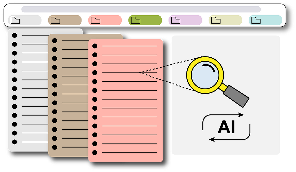
A step-by-step guide for an automated GPT-based bookmark searching pipeline
Image by Author.
Have you encountered moments when searching for a specific bookmark in your Chrome browser only to find that you’re overwhelmed by their sheer number? It becomes quite tedious and draining to sift through your extensive collection of bookmarks.
Bookmark ocean. — Snapshot from author’s Google Chrome bookmark.
Actually, we can simply leave it to ChatGPT which is currently the most popular AI model that can basically answer everything we ask. Imagine, if it can gain access to the bookmarks we have, then bingo! Problem solved! We can then ask it to give us the specific link we want from the entire bookmark storage, like the following GIF:
Showcasing the usage of the AI assistant. — GIF from screen recording.
To achieve this, I built a real-time pipeline to update the Chrome bookmarks into a vector database that ChatGPT will use as the context for our questions. I will explain in this article step by step how to build such a pipeline and you will eventually have your own one too!
Features
Before we begin, let’s count the advantages of it:
Unlike traditional search engines (like the one in Chrome bookmark manager), AI models can have a good semantic understanding of each title. If you forget the exact keyword when searching bookmarks, you can simply draw a rough outline and ChatGPT can get it! It can even understand titles in a different language. Truly remarkable.
What ChatGPT can do. — Snapshot from the AI assistant interfaceWhen the Chrome bookmark search engine fails. — Snapshot from author’s Google Chrome bookmark manager
2. Everything is automatically up-to-date. Each newly added bookmark will be automatically reflected in the AI knowledge database simply within a few minutes.
Pipeline Overview
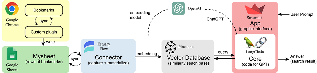
All the components in the pipeline. — Image by Author.
Here you can see the role of each component in our pipeline. The Chrome bookmarks are extracted into rows of a Google Sheet using our customized Chrome plugin. The Estuary Flow gets (or captures) all the sheet data which will then be vectorized (or materialized) by an embedding model using OpenAI API. All the embeddings (each vector corresponds to each row of the sheet — i.e. each single bookmark) will be retrieved and stored in the Pinecone vector database. After that, the user can give prompts to the built app using Streamlit and LangChain (e.g. “Are there links for dinov2?”). It will first retrieve some similar embeddings from Pinecone (getting a context/several potential bookmark options) and combine them with the user’s question as input to ChatGPT. Then ChatGPT will consider every possible bookmark and give a final answer to you. This process is also called RAG: Retrieval Augmented Generation.
In the following parts, we will see how to build such a pipeline step by step.
To transport bookmarks into a Google Sheet for further processing, we need to build a customized Chrome plugin (or extension) first.
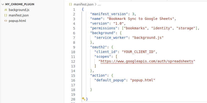
Code structure overview for a Chrome plugin. — Snapshot from author’s vscode.
The most important file for a Chrome extension is the manifest.json, which defines the high-level structure and behavior of the plugin. Here we add the necessary permissions to use the bookmark API from Google Chrome and track the changes in the bookmarks. We also have a field for oauth2 authentication because we will use the Google Sheet API. You will need to put your own client_id in this field. You can mainly follow the Set up your environment sectionin this link to get the client_id and a Google Sheet API key (we will use it later). Something you should notice is:
In OAuth consent screen, you need to add yourself (Gmail address) as the test user. Otherwise, you will not be allowed to use the APIs.
In Create OAuth client ID, the application type you should choose is Chrome extension (not the Web application as in the quickstart link). The Item ID needed to be specified is the plugin ID (we will have it when we load our plugin and you can find it in the extension manager).
The blurred part is the Item ID. — Snapshot from author’s Google Chrome extension manager.
The core functional file is background.js, which can do all the syncs in the background. I’ve prepared the code for you in the GitHub link, the only thing you need to change is the spreadsheetId at the start of the javascript file. This id you can identify it in the sharing link of your created Google Sheet (after d/ and before /edit, and yes you need to manually create a Google Sheet first!):
The main logic of the code is to listen to any change in your bookmarks and refresh (clear + write) your Sheet file with all the bookmarks you have when the plugin is triggered (e.g. when you add a new bookmark). It writes the id, title, and URL of each bookmark into a separate row in your specified Google Sheet.
What it looks like in your Google Sheet. — Snapshot from author’s Google Sheet.
The last file popup.html is basically not that useful as it only defines the content it shows in the popup window when you click the plugin button in your Chrome browser.
After you make sure all the files are in a single folder, now you are ready to upload your plugin:
Go to the Extensions>Manage Extensions of your Chrome browser, and turn on the Developer mode on the top right of the page.
Click the Load unpacked and choose the code folder. Then your plugin will be uploaded and running. Click the hyperlink service worker to see the printed log info from the code.
Once uploaded, the plugin will stay operational as long as the Chrome browser is open. And it’ll also automatically start running when you re-open the browser.
Setting up Estuary Flow and Pinecone
Estuary Flow is basically a connector that syncs the database with the data source you provided. In our case, when Estuary Flow syncs data from a Google Sheet into a vector database — Pinecone, it will also call an embedding model to transform the data into embedding vectors which will then be stored in the Pinecone database.
But please pay attention! Because the Estuary Flow and Pinecone are in fast development. Some points in the video have changed by now, which may cause confusion. Here I list some updates to the video so that you can replicate everything easily:
1.(Estuary Flow>create Capture) In row batch size, you may set some larger numbers according to the total row numbers in your Google Sheet for bookmarks. (e.g. set it to 600 if you’ve already got 400+ rows of bookmarks)
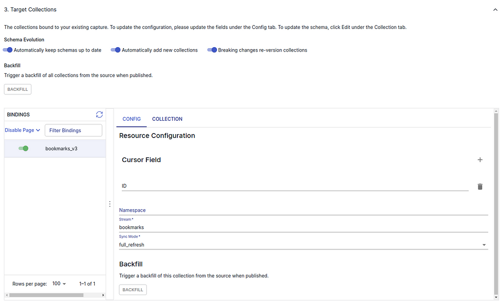
2. (Estuary Flow>create Capture) When setting Target Collections, delete the cursor field “row_id” and add a new one “ID” like the following screenshot. You can keep the namespace empty.
Change Cursor Field. — Snapshot from the Sources on Estuary Flow (April 2024)
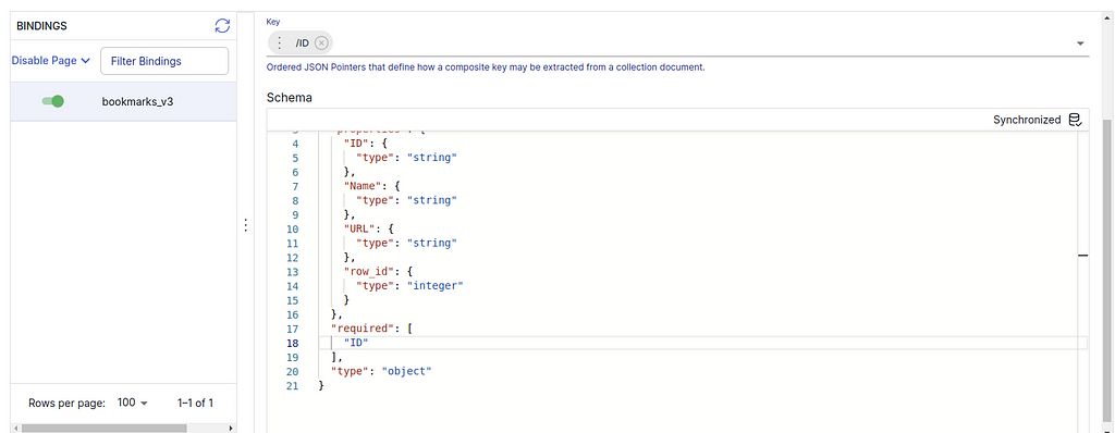
3. (Estuary Flow>create Capture) Then switch to the COLLECTION subtab, press EDIT to change the Key from /row_id to /ID. And you should also change the “required” field of the schema code to “ID” like the following:
Change Key and Schema. — Snapshot from the Sources on Estuary Flow (April 2024)
After “SAVE AND PUBLISH”, you can see that Collections>{your collection name}>Overview>Data Preview will show the correct ID of each bookmark.
4. (Estuary Flow>create Capture) In the last step, you can see an Advanced Specification Editor (in the bottom of the page). Here you can add a field “interval”: 10m to decrease the refresh rate to per 10 minutes (default setting is per 5 minutes if not specified). Each refresh will call the OpenAI embedding model to redo all the embedding which will cost some money. Decreasing the rate is to save half of the money. You can ignore the “backfill” field.
Specify the interval. — Snapshot from the Sources on Estuary Flow (April 2024)
5. (Estuary Flow>create Materialization) The Pinecone environment is typically “gcp-starter” for a free-tier Pinecone index or like “us-east-1-aws” for standard-plan users (I don’t use serverless mode in Pinecone because the Estuary Flow has not yet provided a connector for the Pinecone serverless mode). The Pinecone index is the index name when you create the index in Pinecone.
6. (Estuary Flow>create Materialization) Here are some tricky parts.
First, you should select the source capture using the blue button “SOURCE FROM CAPTURE” and then leave the Pinecone namespace in “CONFIG” EMPTY (the free tier of Pinecone must have an empty namespace).
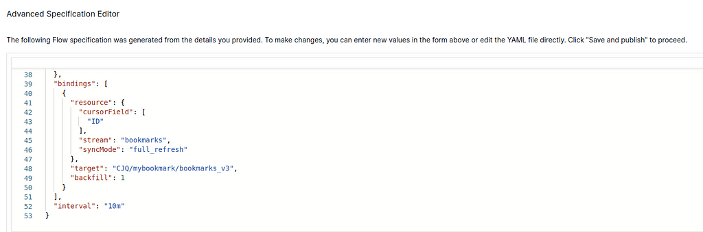
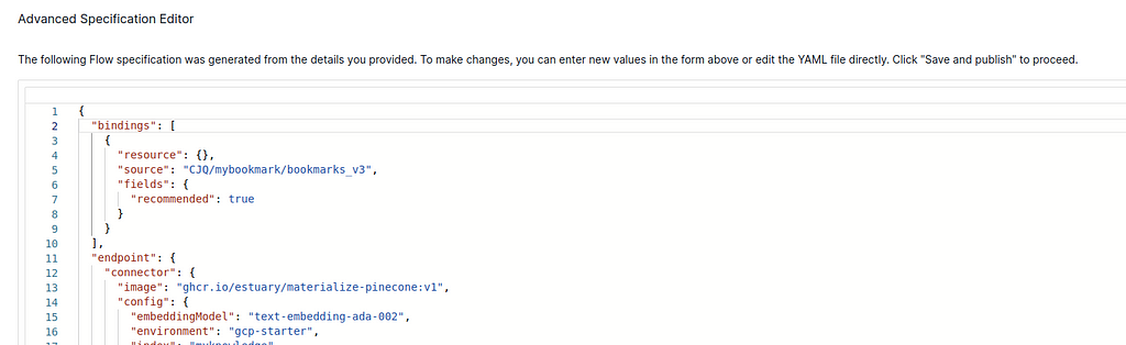
Second, after pressing “NEXT”, in the emerged Advanced Specification Editor of the materialization, you must make sure that the “bindings” field is NOT EMPTY. Fill in the content as in the following screenshot if it is empty or the field does not exist, otherwise, it won’t send anything to Pinecone. Also, you need to change the “source” field using your own Collection path (same as the “target” in the previous screenshot). If some errors pop up after you press “NEXT” and before you can see the editor, press “NEXT” again, and you will see the Advanced Specification Editor. Then you can specify the “bindings” and press “SAVE AND PUBLISH”. Everything should be ok after this step. The errors occur because we didn’t specify the “bindings” before.
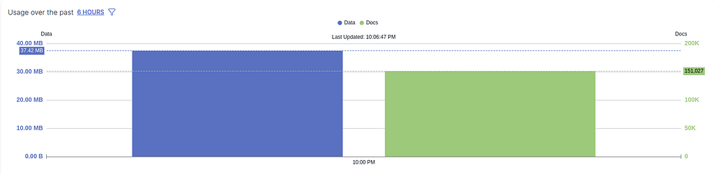
If there is another error message coming up after you have published everything and just returned to the Destination page telling you that you have not added a collection, simply ignore it as long as you see the usage is not zero in the OVERVIEW histogram (see the following screenshots). The histogram basically means how much data it has sent to Pinecone.
Make sure the “bindings” field is filled in like this. — Snapshot from the Destinations on Estuary Flow (April 2024)
Don’t panic about the error, press “NEXT” again. — Snapshot from the Destinations on Estuary Flow (April 2024)Make sure the usage in OVERVIEW is not empty. — Snapshot from the Destinations on Estuary Flow (April 2024)
7. (Pinecone>create index) Pinecone has come up with serverless index mode (free but not supported by Estuary Flow yet) but I don’t use it in this project. Here we still use the pod-based option (not free anymore since last checked on April 14, 2024) which is well enough for our bookmark embedding storage. When creating an index, all you need is to set the index name and dimensions.
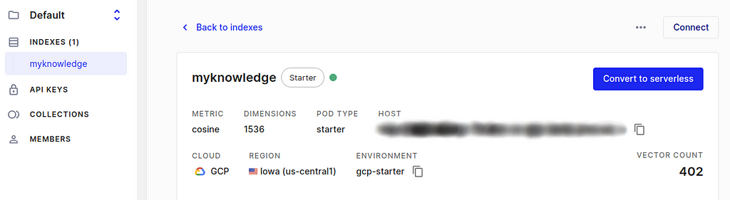
8. (Pinecone>Indexes>{Your index}) After you finish the creation of the Pinecone index and make sure the index name and environment are filled in correctly in the materialization of Estuary Flow, you are set. In the Pincone console, go to Indexes>{Your index} and you should see the vector count showing the total number of your bookmarks. It may take a few minutes until the Pinecone receives information from Estuary Flow and shows the correct vector count.
Here I have 402 bookmarks, so the vector count shows 402. — Snapshot from Pinecone (April 2024)
Building your own App with Streamlit and Langchain
We are almost there! The last step is to build a beautiful interface just like the original ChatGPT. Here we use a very convenient framework called Streamlit, with which we can build an app in only a few lines of code. Langchain is also a user-friendly framework for using any large language model with minimum code.
I’ve also prepared the code for this App for you. Follow the installation and usage guide in the GitHub link and enjoy!
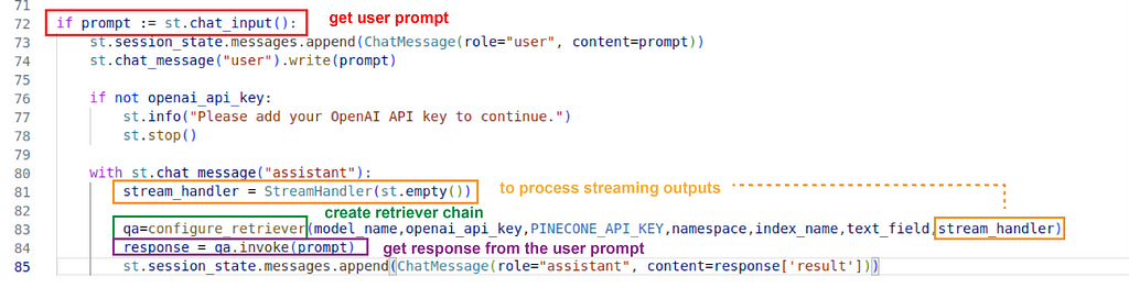
The main logic of the code is:
get user prompt → create a retriever chain with ChatGPT and Pinecone → input the prompt to the chain and get a response → stream the result to the UI
The core part of the code. — Snapshot from author’s vscode.
Please notice, that because the Langchain is in development, the code may be deprecated if you use a newer version other than the stated one in requirements.txt. If you want to dig deeper into Langchain and use another LLM for this bookmark searching, feel free to look into the official documents of Langchain.
Outro
This is the first tutorial post I’ve ever written. If there is anything unclear that needs to be improved or clarified, feel free to leave messages.
We use cookies on our website to give you the most relevant experience by remembering your preferences and repeat visits. By clicking “Accept”, you consent to the use of ALL the cookies.
This website uses cookies to improve your experience while you navigate through the website. Out of these, the cookies that are categorized as necessary are stored on your browser as they are essential for the working of basic functionalities of the website. We also use third-party cookies that help us analyze and understand how you use this website. These cookies will be stored in your browser only with your consent. You also have the option to opt-out of these cookies. But opting out of some of these cookies may affect your browsing experience.
Necessary cookies are absolutely essential for the website to function properly. These cookies ensure basic functionalities and security features of the website, anonymously.
Cookie
Duration
Description
cookielawinfo-checkbox-analytics
11 months
This cookie is set by GDPR Cookie Consent plugin. The cookie is used to store the user consent for the cookies in the category "Analytics".
cookielawinfo-checkbox-functional
11 months
The cookie is set by GDPR cookie consent to record the user consent for the cookies in the category "Functional".
cookielawinfo-checkbox-necessary
11 months
This cookie is set by GDPR Cookie Consent plugin. The cookies is used to store the user consent for the cookies in the category "Necessary".
cookielawinfo-checkbox-others
11 months
This cookie is set by GDPR Cookie Consent plugin. The cookie is used to store the user consent for the cookies in the category "Other.
cookielawinfo-checkbox-performance
11 months
This cookie is set by GDPR Cookie Consent plugin. The cookie is used to store the user consent for the cookies in the category "Performance".
viewed_cookie_policy
11 months
The cookie is set by the GDPR Cookie Consent plugin and is used to store whether or not user has consented to the use of cookies. It does not store any personal data.
Functional cookies help to perform certain functionalities like sharing the content of the website on social media platforms, collect feedbacks, and other third-party features.
Performance cookies are used to understand and analyze the key performance indexes of the website which helps in delivering a better user experience for the visitors.
Analytical cookies are used to understand how visitors interact with the website. These cookies help provide information on metrics the number of visitors, bounce rate, traffic source, etc.
Advertisement cookies are used to provide visitors with relevant ads and marketing campaigns. These cookies track visitors across websites and collect information to provide customized ads.