EVs are getting more popular, but there’s more to their warranties than those for traditional cars. Here’s what you need to know about EV battery warranties.
The US House of Representatives passed a bill on Saturday that could either see TikTok banned in the country or force its sale. A revised version of the bill, which previously passed the House in March but later stalled in Senate, was roped in with a foreign aid package this time around, likely meaning it will now be treated as a higher priority item. The bill originally gave TikTok’s Chinese parent company, ByteDance, six months to sell the app if it’s passed into law or TikTok would be banned from US app stores. Under the revised version, ByteDance would have up to a year to divest.
The bill passed with a vote of 360-58 in the House, according to AP. It’ll now move on to the Senate, which could vote on it as soon as days from now. President Joe Biden has previously said he would support the bill if Congress passes it. The bill paints TikTok as a national security threat due to its ties to China. There are roughly 170 million US users on the app, at least according to TikTok, and ByteDance isn’t expected to let them go without a fight.
In a statement posted on X earlier this week, the TikTok Policy account said such a law would “trample the free speech rights” of these users, “devastate 7 million businesses, and shutter a platform that contributes $24 billion to the U.S. economy, annually.” Critics of the bill have also argued that banning TikTok would do little in the way of actually protecting Americans’ data.
This article originally appeared on Engadget at https://www.engadget.com/house-votes-in-favor-of-bill-that-could-ban-tiktok-sending-it-onward-to-senate-185140206.html?src=rss
Another round of price cuts has shaved $2,000 off the starting prices of Tesla’s Model Y, Model X and Model S for buyers in the US. The company’s North America branch posted on X about the change Friday night, at the same time announcing that Tesla is ditching its referral program benefits in all markets. According to Tesla, the “current referral program benefits will end after April 30.”
Tesla’s Model Y now starts at $42,990 for the rear-wheel drive base model, $47,990 for the Model Y Long Range or $51,490 for the Model Y Performance. The base Model S has dropped to $72,990 while the Model S Plaid now starts at $87,990. The Model X starts at $77,990 (base) or $92,990 (Plaid). The changes come during a rocky few weeks for the company, which just issued a recall for Cybertrucks over possible issues with the accelerator pedal, reportedly laid off 10 percent of its employees and reported a decline in deliveries for the first quarter.
This article originally appeared on Engadget at https://www.engadget.com/tesla-cuts-model-y-x-and-s-prices-in-the-us-and-says-its-ending-the-referral-program-172311662.html?src=rss
Intel’s formidable 288 core CPU now has a proper family name — Granite Rapids and Sierra Forest are Xeon 6 processors but is it just becoming too confusing?
Originally appeared here:
Intel’s formidable 288 core CPU now has a proper family name — Granite Rapids and Sierra Forest are Xeon 6 processors but is it just becoming too confusing?
Creating training data for image segmentation tasks remains a challenge for individuals and small teams. And if you are a student researcher like me, finding a cost-efficient way is especially important. In this post, I will talk about one solution that I used in my capstone project where a team of 9 people successfully labeled 400+ images within a week.
Thanks to Politecnico de Milano Gianfranco Ferré Research Center, we obtained thousands of fashion runway show images from Gianfranco Ferré’s archival database. To explore, manage, enrich, and analyze the database, I employed image segmentation forsmarter cataloging and fine-grained research. Image segmentation of runway show photos also lays the foundation for creating informative textual descriptions for better search engine and text-to-image generative AI approaches. Therefore, this blog will detail:
how to create your own backend with label studio, on top of the existing segment anything backend, for semiautomatic image segmentation labeling,
how to host on Google Cloud Platform for group collaboration, and
how to employ Google Cloud Storage buckets for data versioning.
Code in this post can be found in this GitHub repo.
Overview
Goal
Segment and identify the names and typologies of fashion clothing items in runway show images, as shown in the first image.
Why semiautomatic?
Wouldn’t it be nice if a trained segmentation model out there could perfectly recognize every piece of clothing in the runway show images? Sadly, there isn’t one. There exist trained models tailored to fashion or clothing images but nothing can match our dataset perfectly. Each fashion designer has their own style and preferences for certain clothing items and their color and texture, so even if a segmentation model can be 60% accurate, we call it a win. Then, we still need humans in the loop to correct what the segmentation model got wrong.
Entering Label Studio
Label Studio provides an open-source, customizable, and free-of-charge community version for various types of data labeling. One can create their own backend, so I can connect the Label Studio frontend to the trained segmentation model (mentioned above) backend for labelers to further improve upon the auto-predictions. Furthermore, Label Studio already has an interface that looks somewhat similar to Photoshop and a series of segmentation tools that can come in handy for us:
Segment Anything backend which harnesses the power of Meta’s SAM and allows you to recognize the object within a bounding box you draw.
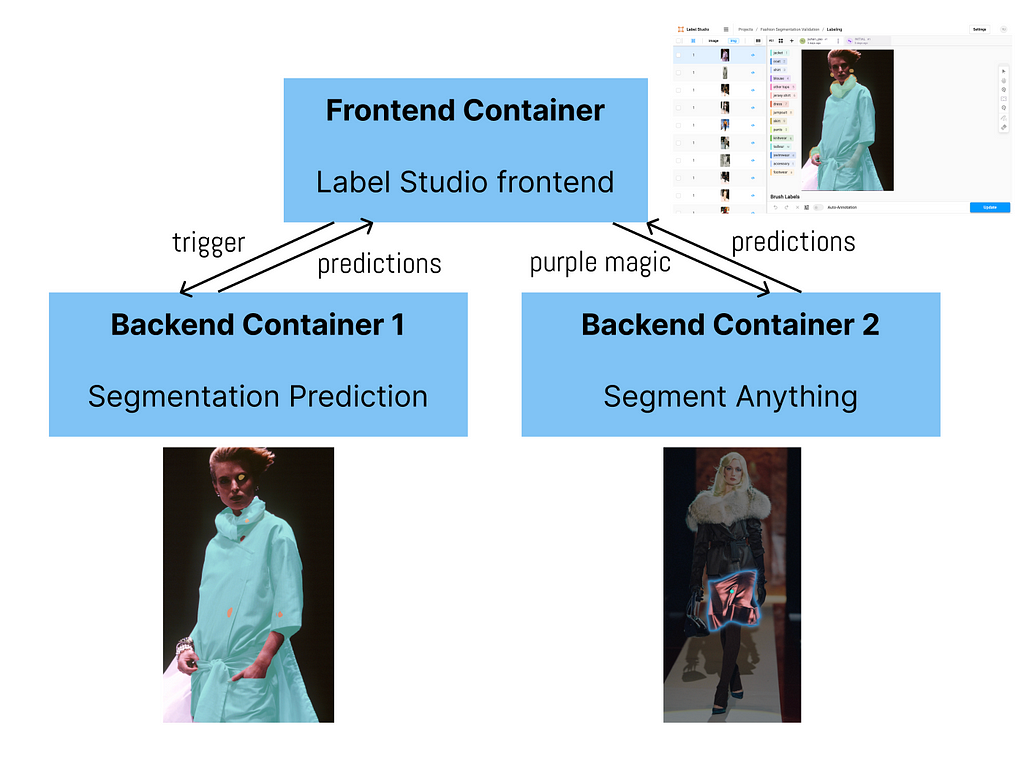
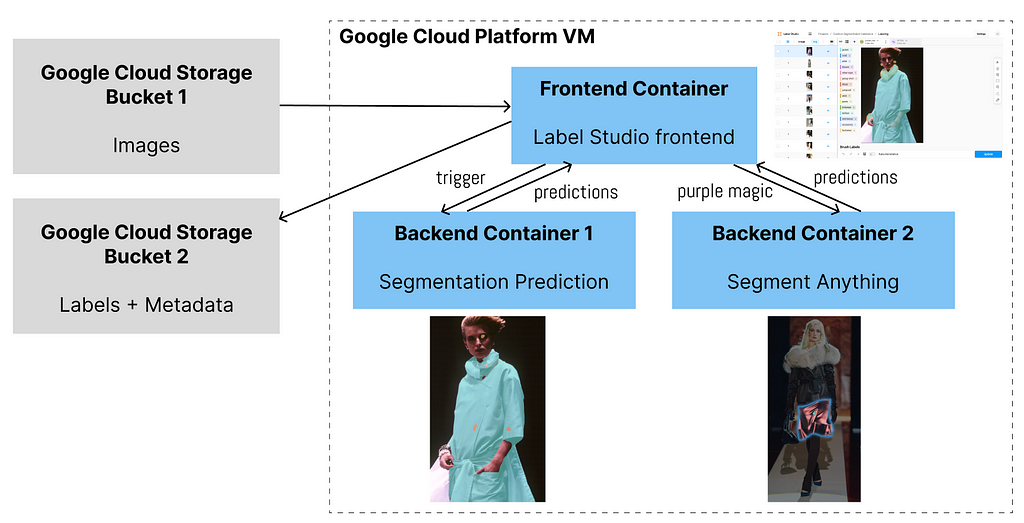
1 frontend + 2 backends
So far, we want 2 backends to be connected to the frontend. One backend can do the segmentation prediction and the second can speed up labelers’ modification if the predictions are wrong.
Image by Author
Implementation (Local)
Now, let’s fire up the app locally. That is, you will be able to use the app on your laptop or local machine completely for free but you are not able to invite your labeling team to collaborate on their laptops yet. We will talk about teamwork with GCP in the next section.
1. Install git and docker & download backend code
If you don’t have git or docker on your laptop or local machine yet, please install them. (Note: you can technically bypass the step of installing git if you download the zip file from this GitHub repo. If you do so, skip the following.)
Then, open up your terminal and clone this repo to a directory you want.
If you open up the label-studio-customized-ml-backend folder in your code editor, you can see the majority are adapted from the Label Studio ML backend repo, but this directory also contains frontend template code and SDK code adapted from Label Studio SDK.
2. Set up frontend to get access token
Following the official guidelines of segment anything, do the following in your terminal:
cd label-studio-customized-ml-backend/label_studio_ml/examples/segment_anything_model
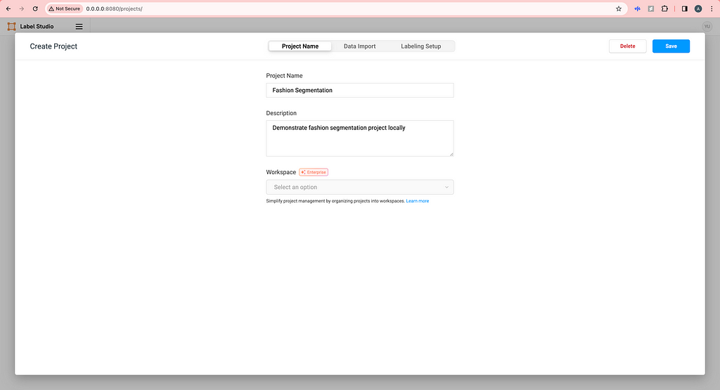
Then, open your browser and type http://0.0.0.0:8080/ and you will see the frontend of Label Studio. Proceed to sign up with your email address. Now, there is no project yet so we need to create our first project by clicking Create Project. Create a name and description (optional) for your project.
Image by Author
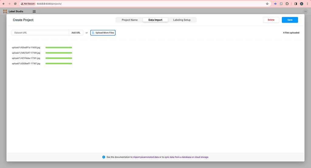
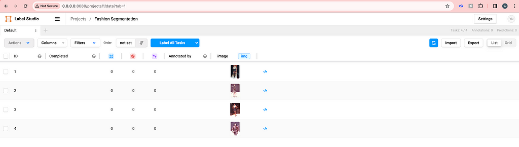
Upload some images locally. (We will talk about how to use cloud storage later.)
Image by Author
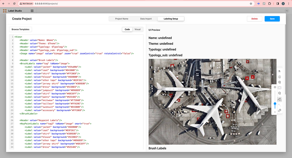
For Labeling Setup, click on Custom template on the left and copy-paste the HTML code from the label-studio-customized-ml-backend/label_studio_frontend/view.html file. You do not need the four lines of Headers if you don’t want to show image metadata in the labeling interface. Feel free to modify the code here to your need or click Visual to add or delete labels.
Image by Author
Now, click Save and your labeling interface should be ready.
Image by Author
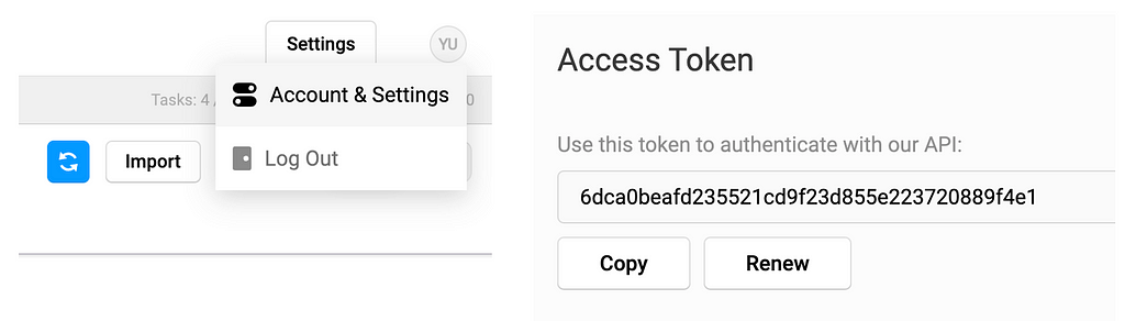
On the top right, click on the user setting icon and click Account & Setting and then you should be able to copy your access token.
Image by Author
3. Set up backend containers
In the label-studio-customized-ml-backend directory, there are many many backends thanks to the Label Studio developers. We will be using the customized ./segmentation backend for segmentation prediction (container 1) and the ./label_studio_ml/examples/segment_anything_model for faster labeling (container 2). The former will use port 7070 and the latter will use port 9090, making it easy to distinguish from the frontend port 8080.
Now, paste your access token to the 2 docker-compose.yml files in ./segmentationand ./label_studio_ml/examples/segment_anything_model folders.
Open up a new terminal and you cd into the segment_anything_model directory as you did before. Then, fire up the segment anything container.
cd label-studio-customized-ml-backend/label_studio_ml/examples/segment_anything_model

docker build . -t sam:latest
docker compose up
Then, open up another new terminal cd into the segmentation directory and fire up the segmentation prediction container.
cd label-studio-customized-ml-backend/segmentation

docker build . -t seg:latest
docker compose up
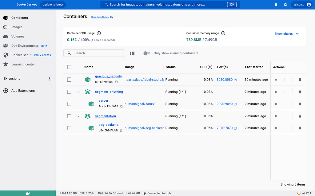
As of now, we have successfully started all 3 containers and you can double-check.
Image by Author
4. Connect containers
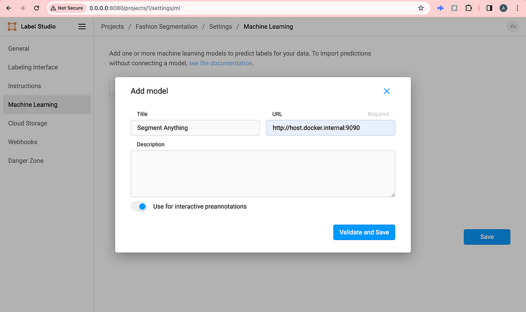
Before, what we did with the access token was helping us connect containers already, so we are almost done. Now, go to the frontend you started a while back and click Settings in the top right corner. Click Machine Learning on the left and click Add Model.
Image by Author
Be sure to use the URL with port 9090 and toggle on interactive preannotation. Finish adding by clicking Validate and Save.
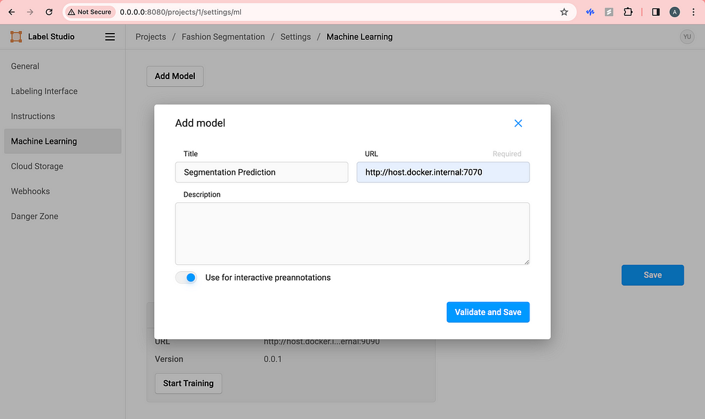
Similarly, do the same with the segmentation prediction backend.
Image by Author
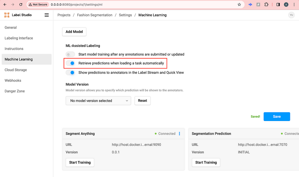
Then, I like to toggle on Retrieve predictions when loading a task automatically. This way, every time we refresh the labeling page, the segmentation predictions will be automatically triggered and loaded.
Image by Author
5. Happy labeling!
Here is a demo of what you should see if you follow the steps above.
If we are not happy with the predictions of let’s say the skirt, we can delete the skirt and use the purple magic (segment anything) to quickly label it.
I’m sure you can figure out how to use the brush, eraser and magic wand on your own!
If you are working solo, you are all set. But if you are wondering how to collaborate with your team without subscribing to Label Studio Enterprise, we need to host everything on cloud.
GCP Deployment
I chose GCP because of education credits, but you can use any cloud of your choice. The point is to host the app on cloud so that anyone in your labeling team can access and use your Label Studio app.
Image by Author
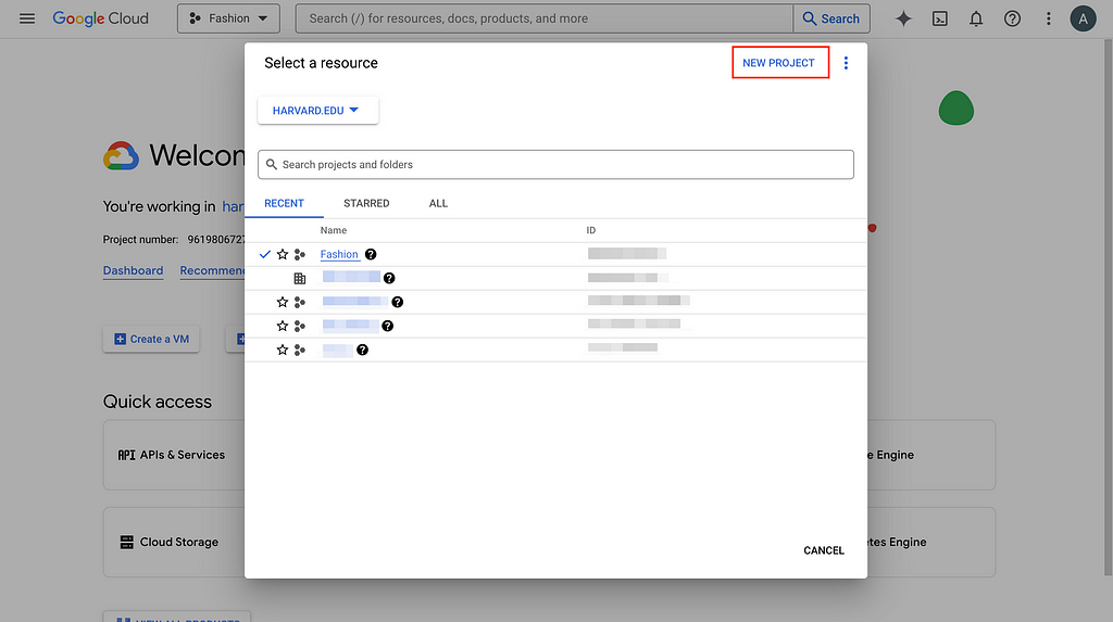
1. Select project/Create new project and set up billing account
Go to GCP console and create a new project if you don’t have an existing one and set up the billing account information as required (unfortunately, cloud costs some money). Here, I will use the Fashion project I created to demonstrate.
Image by Author
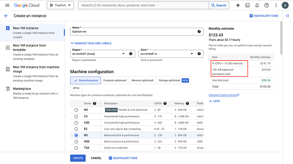
2. Create VM instance
To have a public IP address for labeling teamwork, we need to create a Virtual Machine (VM) on GCP and host everything here. After going to the project you created or selected, search compute engine in the search bar and the first thing that pops up should be VM instances. Click CREATE INSTANCE and choose the setting based on your need.
Image by Author
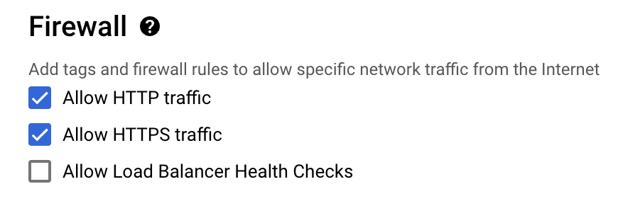
The default 10GB persistent disk will give you problems, so bump it up please. And more importantly, allow HTTP traffic.
Image by Author
It is a bit painful to modify these settings later, so try to think it through before clicking CREATE.
3. Set up VM environment
You can think of a VM as a computer somewhere in the cloud, similar to your laptop, but you can only ask it to do things via the terminal or command line. So now we need to set up everything on the VM the same way we set up everything locally (see previous section).
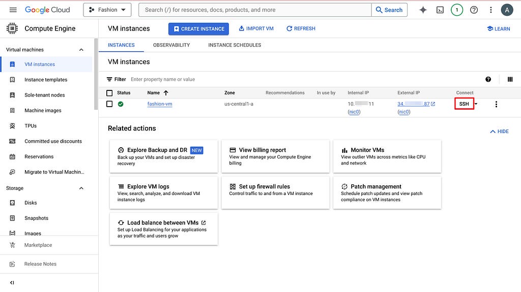
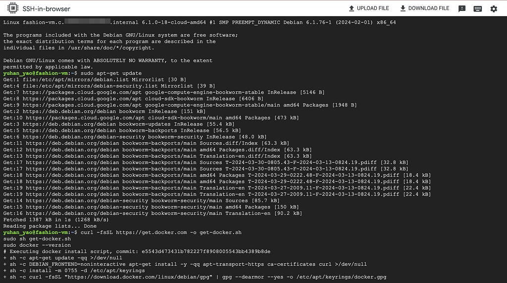
Click SSH, authorize and open up the command line interface.
Image by Author
Do routine update and install docker, docker compose, git and Python.
4. Follow previous section & set up everything on VM
Now, you can follow steps 1–4 in the previous section but there are some changes:
Add sudo when you have docker permission denied error.
If you have data permission error, modify permission using something like sudo chmod -R 777 mydata. And then you should be able to run your frontend container.
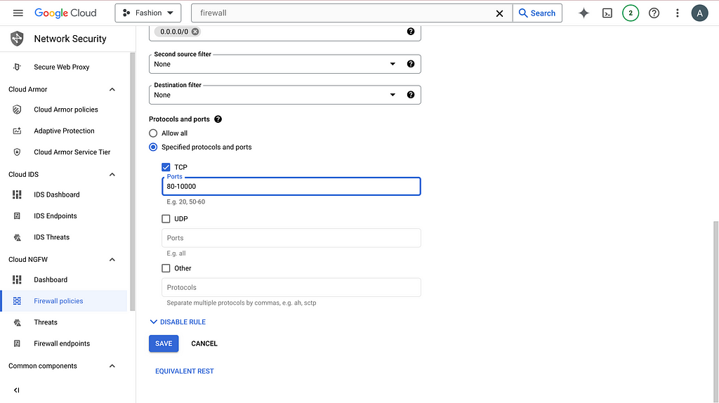
The server is not at http://0.0.0.0:8080 anymore. Instead, swap 0.0.0.0 with the external IP address of your VM. An example is http://34.1.1.87:8080/. You can find the external IP address next to the SSH button you clicked before. However, you probably still cannot access the frontend just yet. You need to search firewall on GCP console and click Firewall (VPC network) and then click default-allow-http. Now, change the setting to the following and you should be able to access the frontend.
Image by Author
4. When editing docker-compose.yml files, apart from copy-pasting access token, also modify the LABEL_STUDIO_HOST. Again, swap host.docker.internal with the VM external IP address. An example is http://34.1.1.87:8080 .
You can then export your labeling results and tailor to your uses.
If you only have a couple of images to label or you are fine with uploading images from local, by all means. But for my project, there are thousands of images, so I prefer using Google Cloud Storage to automate data transferring and data versioning.
GCS Integration
1. Set up GCS buckets
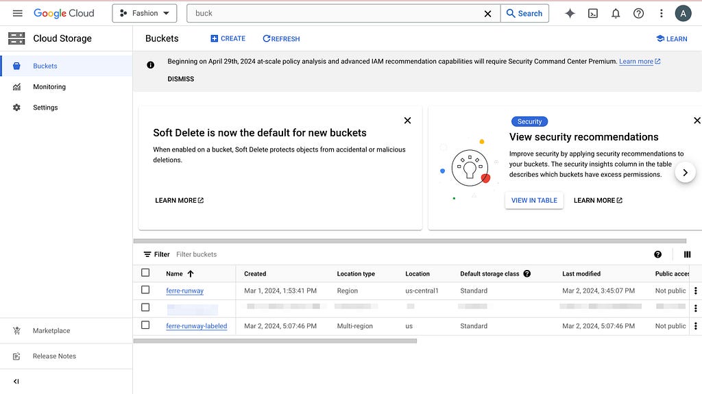
Search bucket in the GCP console and navigate to Cloud Storage buckets. Create 2 buckets: one with your images (source) and another empty (target). The second one will be populated later when you start labeling.
Image by Author
Then, following the official documentation, we need to set up cross-origin resource sharing (CORS) access to the buckets. Click Activate Cloud Shell on the top right, and run the following commands.
gsutil cors set cors-config.json gs://ferre-runway # use your bucket name gsutil cors set cors-config.json gs://ferre-runway-labeled # use your bucket name
If you want to set up data versioning for the labeling results, you can click on the bucket and turn on versioning in PROTECTION.
Image by Author
2. Create & set up service account key
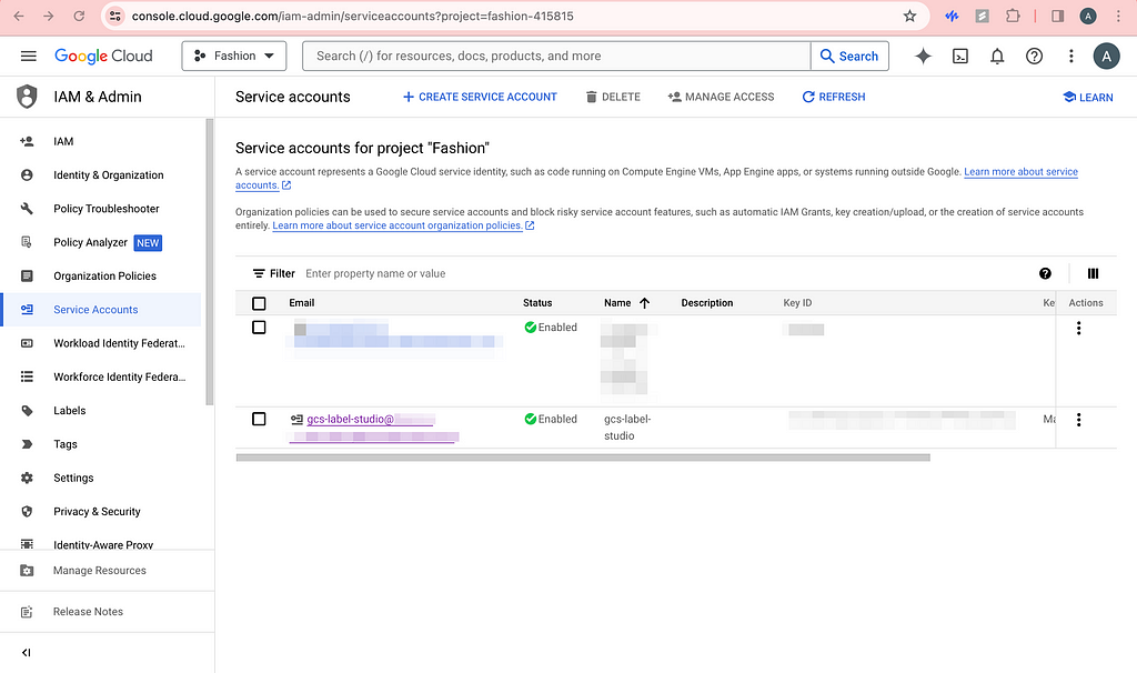
Chances are that you do not want your buckets to be public, then label studio needs authentication to have access to these images. Click CREATE SERVICE ACCOUNT and grant the role of Storage Admin so that we can read and write to the GCS buckets. You should be able to see this service account in the permissions list of the buckets as well.
Image by Author
Now, click on the newly created service account and click KEYS. Now add a new key and be sure to download the JSON file to somewhere safe.
Now, open up your local terminal and encode the JSON file.
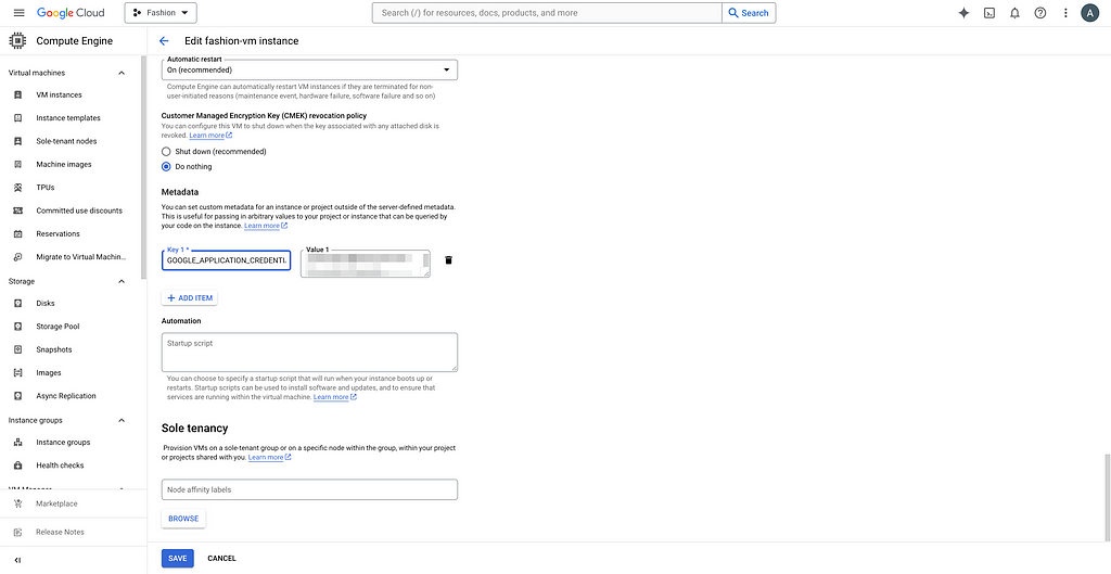
You can see the random character and number string and copy it. We are now pasting it as metadata for the VM. Click on your VM, click EDIT, and add your custom metadata. For example, my key is GOOGLE_APPLICATION_CREDENTIALS_BASE64.
Image by Author
We will then decode the service account key for authentication in our Python code.
3. Rebuild backend containers
Since we modified the docker-compose.yml files, we need to run the new script and rebuild the backend containers.
# Check running containers and their IDs, find the backends you need to kill sudo docker ps
# navigate to the right folders like before and build new containers sudo docker compose up
Now, you should see the new containers.
Image by Author
4. SDK upload images from source bucket
If you simply want to upload the images without metadata, you can skip this section and do the exact same thing as step 5 (see next). By metadata, I mean the useful information for each image on the labeling interface that might help with labeling more accurately.
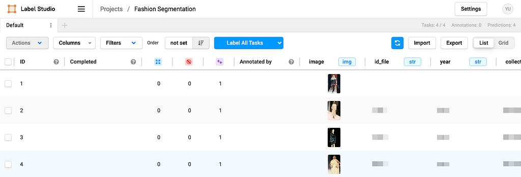
Based on the example from Label Studio SDK repo, you can modify what metadata and how you want to import in the ./label_studio_sdk/annotate_data_from_gcs.ipynb file. After running the python notebook locally, you should be able to see your images and metadata on the frontend.
Image by Author
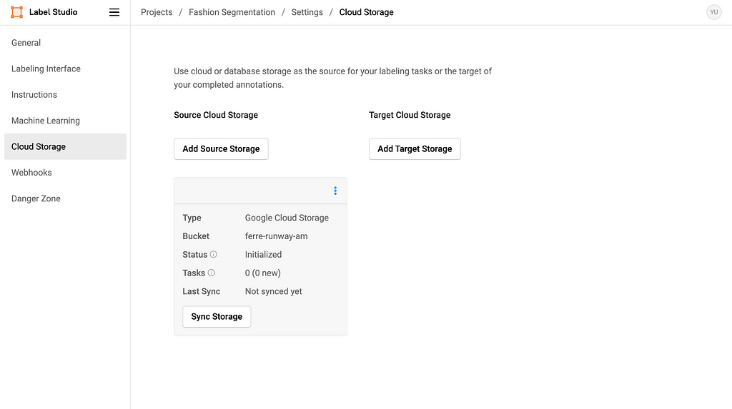
And you should also see the Source Storage bucket in the settings. Do NOT click Sync Storage as it will sync directly from the bucket and mess up the metadata we imported.
Image by Author
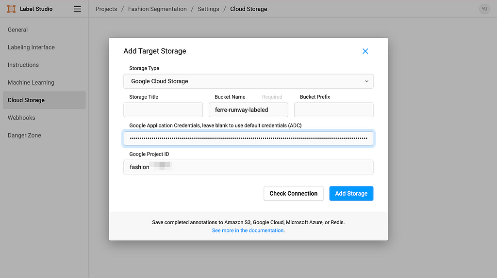
5. Set up Target Storage
Click Add Target Storage, and filling in the information accordingly. Copy-paste your service account key in the Google Application Credentials textbox and you are all set.
Image by Author
Every time you click Sync Storage on the Target Cloud Storage, it will sync the labeling outcome in the format of text into the GCS bucket. After clicking sync once, the process should be trigger automatically when submitting labeling results, but please check if you need to manually sync from time to time just in case.
Happy labeling!
Acknowledgement
It is my pleasure to be a part of Data Shack 2024 in collaboration with Politecnico de Milano Gianfranco Ferré Research Center. I would like to thank Prof. Pavlos Protopapas and Prof. Paola Bertola for your guidance and for making this project happen in the first place. I would like to thank Chris Gumb and Prof. Marco Brambilla for technical support and Prof. Federica Vacca and Dr. Angelica Vandi for domain knowledge expertise in fashion. Finally, I would like to thank my teammates Luis Henrique Simplicio Ribeiro, Lorenzo Campana and Vittoria Corvetti for your help and for figuring things out with me along the way. I also want to give a round of applause to Emanuela Di Stefano, Jacopo Sileo, Bruna Pio Da Silva Rigato, Martino Fois, Xinxi Liu, and Ilaria Trame for your continued support and hard work.
References
11655 Gianfranco Ferré, Ready-To-Wear Collection, Fall-Winter 2004. Courtesy of Gianfranco Ferré Research Center
13215 Gianfranco Ferré, Ready-To-Wear Collection, Spring-Summer 1991. Courtesy of Gianfranco Ferré Research Center
Thank you for reading! I hope this blog has been helpful to you.
Code in this post can be found in this GitHub repo.
Dive into the “Curse of Dimensionality” concept and understand the math behind all the surprising phenomena that arise in high dimensions.
Image from Dall-E
In the realm of machine learning, handling high-dimensional vectors is not just common; it’s essential. This is illustrated by the architecture of popular models like Transformers. For instance, BERT uses 768-dimensional vectors to encode the tokens of the input sequences it processes and to better capture complex patterns in the data. Given that our brain struggles to visualize anything beyond 3 dimensions, the use of 768-dimensional vectors is quite mind-blowing!
While some Machine and Deep Learning models excel in these high-dimensional scenarios, they also present many challenges. In this article, we will explore the concept of the “curse of dimensionality”, explain some interesting phenomena associated with it, delve into the mathematics behind these phenomena, and discuss their general implications for your Machine Learning models.
Note that detailed mathematical proofs related to this article are available on my website as a supplementary extension to this article.
What is the curse of dimensionality?
People often assume that geometric concepts familiar in three dimensions behave similarly in higher-dimensional spaces. This is not the case. As dimension increases, many interesting and counterintuitive phenomena arise. The “Curse of Dimensionality” is a term invented by Richard Bellman (famous mathematician) that refers to all these surprising effects.
What is so special about high-dimension is how the “volume” of the space (we’ll explore that in more detail soon) is growing exponentially. Take a graduated line (in one dimension) from 1 to 10. There are 10 integers on this line. Extend that in 2 dimensions: it is now a square with 10 × 10 = 100 points with integer coordinates. Now consider “only” 80 dimensions: you would already have 10⁸⁰ points which is the number of atoms in the universe.
In other words, as the dimension increases, the volume of the space grows exponentially, resulting in data becoming increasingly sparse.
High-dimensional spaces are “empty”
Consider this other example. We want to calculate the farthest distance between two points in a unit hypercube (where each side has a length of 1):
In 1 dimension (the hypercube is a line segment from 0 to 1), the maximum distance is simply 1.
In 2 dimensions (the hypercube forms a square), the maximum distance is the distance between the opposite corners [0,0] and [1,1], which is √2, calculated using the Pythagorean theorem.
Extending this concept to n dimensions, the distance between the points at [0,0,…,0] and [1,1,…,1] is √n. This formula arises because each additional dimension adds a square of 1 to the sum under the square root (again by the Pythagorean theorem).
Interestingly, as the number of dimensions n increases, the largest distance within the hypercube grows at an O(√n) rate. This phenomenon illustrates a diminishing returns effect, where increases in dimensional space lead to proportionally smaller gains in spatial distance. More details on this effect and its implications will be explored in the following sections of this article.
The notion of distance in high dimensions
Let’s dive deeper into the notion of distances we started exploring in the previous section.
We had our first glimpse of how high-dimensional spaces render the notion of distance almost meaningless. But what does this really mean, and can we mathematically visualize this phenomenon?
Let’s consider an experiment, using the same n-dimensional unit hypercube we defined before. First, we generate a dataset by randomly sampling many points in this cube: we effectively simulate a multivariate uniform distribution. Then, we sample another point (a “query” point) from that distribution and observe the distance from its nearest and farthest neighbor in our dataset.
Here is the corresponding Python code.
def generate_data(dimension, num_points):
    ''' Generate random data points within [0, 1] for each coordinate in the given dimension '''
    data = np.random.rand(num_points, dimension)
    return data


def neighbors(data, query_point):
    ''' Returns the nearest and farthest point in data from query_point '''
    nearest_distance = float('inf')
    farthest_distance = 0
    for point in data:
        distance = np.linalg.norm(point - query_point)
        if distance < nearest_distance:
            nearest_distance = distance
        if distance > farthest_distance:
            farthest_distance = distance
    return nearest_distance, farthest_distance
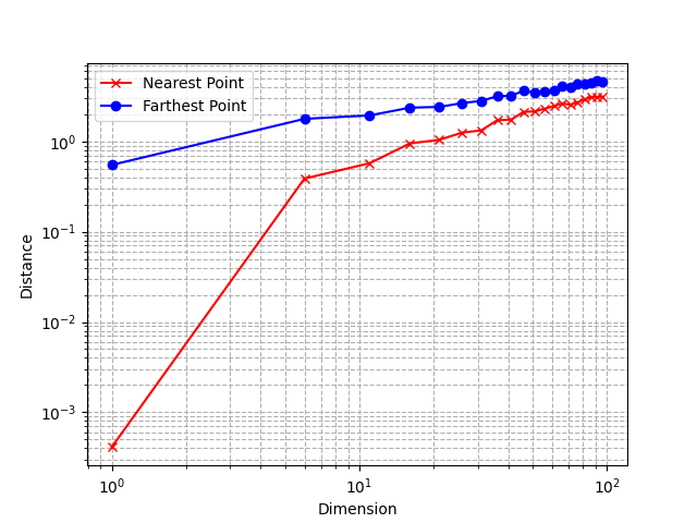
We can also plot these distances:
Distances to nearest and farthest points as n increases (Image by the author)
Using a log scale, we observe that the relative difference between the distance to the nearest and farthest neighbor tends to decrease as the dimension increases.
This is a very unintuitive behavior: as explained in the previous section, points are very sparse from each other because of the exponentially increasing volume of the space, but at the same time, the relative distances between points become smaller.
The notion of nearest neighbors vanishes
This means that the very concept of distance becomes less relevant and less discriminative as the dimension of the space increases. As you can imagine, it poses problems for Machine Learning algorithms that solely rely on distances such as kNN.
The maths: the n-ball
We will now talk about some other interesting phenomena. For this, we’ll need the n-ball. A n-ball is the generalization of a ball in n dimensions. The n-ball of radius R is the collection of points at a distance at most R from the center of the space 0.
Let’s consider a radius of 1. The 1-ball is the segment [-1, 1]. The 2-ball is the disk delimited by the unit circle, whose equation is x² + y² ≤ 1. The 3-ball (what we normally call a “ball”) has the equation x² + y² + z² ≤ 1. As you understand, we can extend that definition to any dimension:
The question now is: what is the volume of this ball? This is not an easy question and requires quite a lot of maths, which I won’t detail here. However, you can find all the details on my website, in my post about the volume of the n-ball.
After a lot of fun (integral calculus), you can prove that the volume of the n-ball can be expressed as follows, where Γ denotes the Gamma function.
For example, with R = 1 and n = 2, the volume is πR², because Γ(2) = 1. This is indeed the “volume” of the 2-ball (also called the “area” of a circle in this case).
However, beyond being an interesting mathematical challenge, the volume of the n-ball also has some very surprising properties.
As the dimension n increases, the volume of the n-ball converges to 0.
This is true for every radius, but let’s visualize this phenomenon with a few values of R.
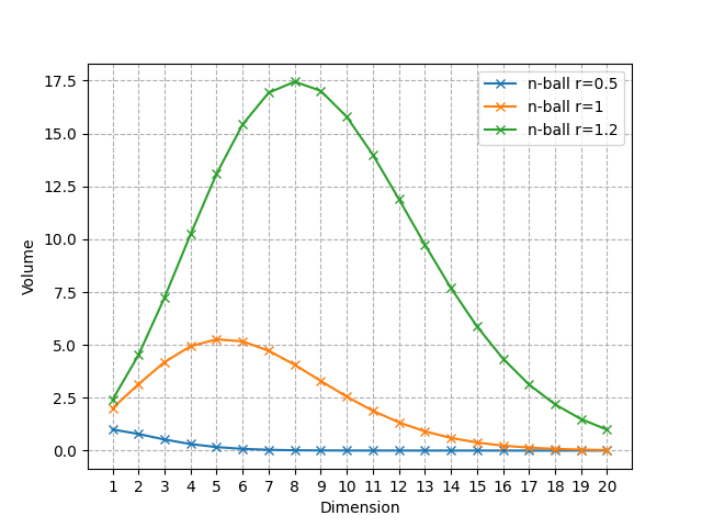
Volume of the n-ball for different radii as the dimension increases (Image by the author)
As you can see, it only converges to 0, but it starts by increasing and then decreases to 0. For R = 1, the ball with the largest volume is the 5-ball, and the value of n that reaches the maximum shifts to the right as R increases.
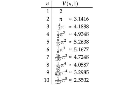
Here are the first values of the volume of the unit n-ball, up to n = 10.
Volume of the unit n-ball for different values of n (Image by the author)
The volume of a high-dimensional unit ball is concentrated near its surface.
For small dimensions, the volume of a ball looks quite “homogeneous”: this is not the case in high dimensions.
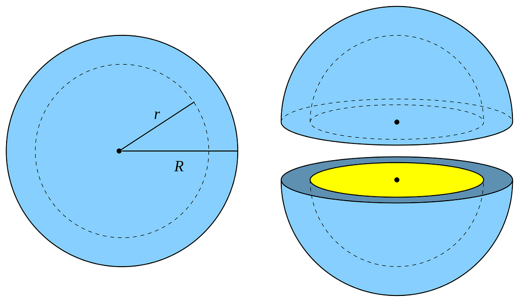
A spherical shell
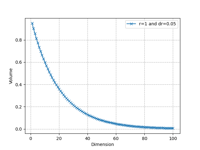
Let’s consider an n-ball with radius R and another with radius R-dR where dR is very small. The portion of the n-ball between these 2 balls is called a “shell” and corresponds to the portion of the ball near its surface(see the visualization above in 3D). We can compute the ratio of the volume of the entire ball and the volume of this thin shell only.
Ratio (total volume / thin shell volume) as n increases (Image by the author)
As we can see, it converges very quickly to 0: almost all the volume is near the surface in high dimensional spaces. For instance, for R = 1, dR = 0.05, and n = 50, about 92.3% of the volume is concentrated in the thin shell. This shows that in higher dimensions, the volume is in “corners”. This is again related to the distortion of the concept of distance we have seen earlier.
Note that the volume of the unit hypercube is 2ⁿ. The unit sphere is basically “empty” in very high dimensions, while the unit hypercube, in contrast, gets exponentially more points. Again, this shows how the idea of a “nearest neighbor” of a point loses its effectiveness because there is almost no point within a distance R of a query point q when n is large.
Curse of dimensionality, overfitting, and Occam’s Razor
The curse of dimensionality is closely related to the overfitting principle. Because of the exponential growth of the volume of the space with the dimension, we need very large datasets to adequately capture and model high-dimensional patterns. Even worse: we need a number of samples that grows exponentially with the dimension to overcome this limitation. This scenario, characterized by many features yet relatively few data points, is particularly prone to overfitting.
Occam’s Razor suggests that simpler models are generally better than complex ones because they are less likely to overfit. This principle is particularly relevant in high-dimensional contexts (where the curse of dimensionality plays a role) because it encourages the reduction of model complexity.
Applying Occam’s Razor principle in high-dimensional scenarios can mean reducing the dimensionality of the problem itself (via methods like PCA, feature selection, etc.), thereby mitigating some effects of the curse of dimensionality. Simplifying the model’s structure or the feature space helps in managing the sparse data distribution and in making distance metrics more meaningful again. For instance, dimensionality reduction is a very common preliminary step before applying the kNN algorithm. More recent methods, such as ANNs (Approximate Nearest Neighbors) also emerge as a way to deal with high-dimensional scenarios.
Blessing of dimensionality?
Image by Dall-E
While we’ve outlined the challenges of high-dimensional settings in machine learning, there are also some advantages!
High dimensions can enhance linear separability, making techniques like kernel methods more effective.
Additionally, deep learning architectures are particularly adept at navigating and extracting complex patterns from high-dimensional spaces.
As always with Machine Learning, this is a trade-off: leveraging these advantages involves balancing the increased computational demands with potential gains in model performance.
Conclusion
Hopefully, this gives you an idea of how “weird” geometry can be in high-dimension and the many challenges it poses for machine learning model development. We saw how, in high-dimensional spaces, data is very sparse but also tends to be concentrated in the corners, and distances lose their usefulness. For a deeper dive into the n-ball and mathematical proofs, I encourage you to visit the extended of this article on my website.
While the “curse of dimensionality” outlines significant limitations in high-dimensional spaces, it’s exciting to see how modern deep learning models are increasingly adept at navigating these complexities. Consider the embedding models or the latest LLMs, for example, which utilize very high-dimensional vectors to more effectively discern and model textual patterns.
Want to learn more about Transformers and how they transform your data under the hood? Check out my previous article:
We use cookies on our website to give you the most relevant experience by remembering your preferences and repeat visits. By clicking “Accept”, you consent to the use of ALL the cookies.
This website uses cookies to improve your experience while you navigate through the website. Out of these, the cookies that are categorized as necessary are stored on your browser as they are essential for the working of basic functionalities of the website. We also use third-party cookies that help us analyze and understand how you use this website. These cookies will be stored in your browser only with your consent. You also have the option to opt-out of these cookies. But opting out of some of these cookies may affect your browsing experience.
Necessary cookies are absolutely essential for the website to function properly. These cookies ensure basic functionalities and security features of the website, anonymously.
Cookie
Duration
Description
cookielawinfo-checkbox-analytics
11 months
This cookie is set by GDPR Cookie Consent plugin. The cookie is used to store the user consent for the cookies in the category "Analytics".
cookielawinfo-checkbox-functional
11 months
The cookie is set by GDPR cookie consent to record the user consent for the cookies in the category "Functional".
cookielawinfo-checkbox-necessary
11 months
This cookie is set by GDPR Cookie Consent plugin. The cookies is used to store the user consent for the cookies in the category "Necessary".
cookielawinfo-checkbox-others
11 months
This cookie is set by GDPR Cookie Consent plugin. The cookie is used to store the user consent for the cookies in the category "Other.
cookielawinfo-checkbox-performance
11 months
This cookie is set by GDPR Cookie Consent plugin. The cookie is used to store the user consent for the cookies in the category "Performance".
viewed_cookie_policy
11 months
The cookie is set by the GDPR Cookie Consent plugin and is used to store whether or not user has consented to the use of cookies. It does not store any personal data.
Functional cookies help to perform certain functionalities like sharing the content of the website on social media platforms, collect feedbacks, and other third-party features.
Performance cookies are used to understand and analyze the key performance indexes of the website which helps in delivering a better user experience for the visitors.
Analytical cookies are used to understand how visitors interact with the website. These cookies help provide information on metrics the number of visitors, bounce rate, traffic source, etc.
Advertisement cookies are used to provide visitors with relevant ads and marketing campaigns. These cookies track visitors across websites and collect information to provide customized ads.