Tag: tech

From data to decisions: maximizing rewards with policy improvement methods for optimal strategies

Introduction

Reinforcement learning is a domain in machine learning that introduces the concept of an agent who must learn optimal strategies in complex environments. The agent learns from its actions that result in rewards given the environment’s state. Reinforcement learning is a difficult topic and differs significantly from other areas of machine learning. That is why it should only be used when a given problem cannot be solved otherwise.

The incredible flexibility of reinforcement learning is that the same algorithms can be used to make the agent adapt to completely different, unknown, and complex conditions.

Note. To fully understand the ideas included in this article, it is highly recommended to be familiar with the main concepts of reinforcement learning introduced in the first part of this article series.

Reinforcement Learning, Part 1: Introduction and Main Concepts

About this article

In Part 1, we have introduced the main concepts of reinforcement learning: the framework, policies and value functions. The Bellman equation that recursively establishes the relationship of value functions is the backbone of modern algorithms. We will understand its power in this article by learning how it can be used to find optimal policies.

This article is based on Chapter 4 of the book “Reinforcement Learning” written by Richard S. Sutton and Andrew G. Barto. I highly appreciate the efforts of the authors who contributed to the publication of this book.

Solving Bellman equation

Let us imagine that we perfectly know the environment’s dynamics that contains |S| states. Action transition probablities are given by a policy π. Given that, we can solve the Bellman equation for the V-function for this environment that will, in fact, represent a system of linear equations with |S| variables (in case of the Q-function there will be |S| x |A| equations).

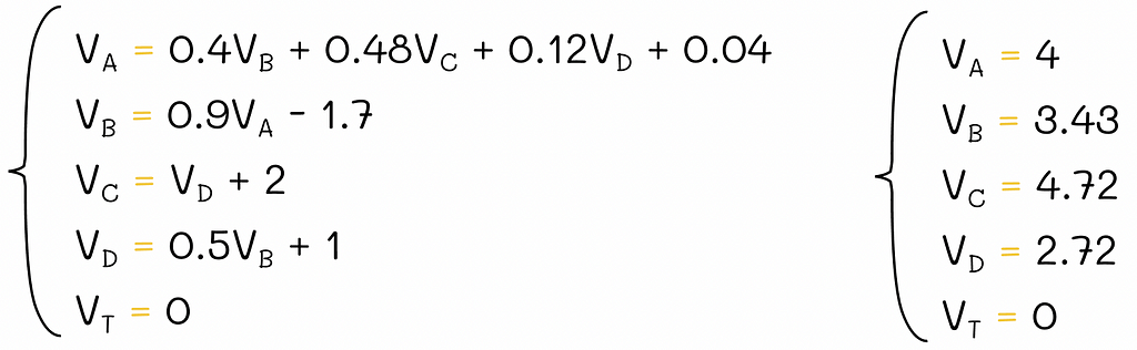
The solution to that system of equations corresponds to v-values for every state (or q-values for every pair (state, pair)).

Example

Let us have a look at a simple example of an environment with 5 states where T is a terminal state. Numbers in blue represent transition probabilities while number in red represent rewards received by the agent. We will also assume that the same action chosen by the agent in the state A (represented by the horizontal arrow with probability p = 0.6) leads to either C or D with different probabilities (p = 0.8 and p = 0.2).

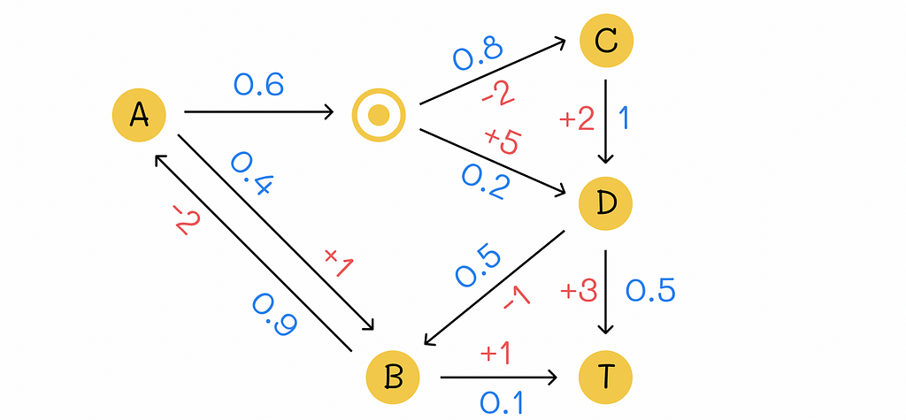
Since the environment contains |S| = 5 states, to find all v-values, we will have to solve a system of equations consisting of 5 Bellman equations:

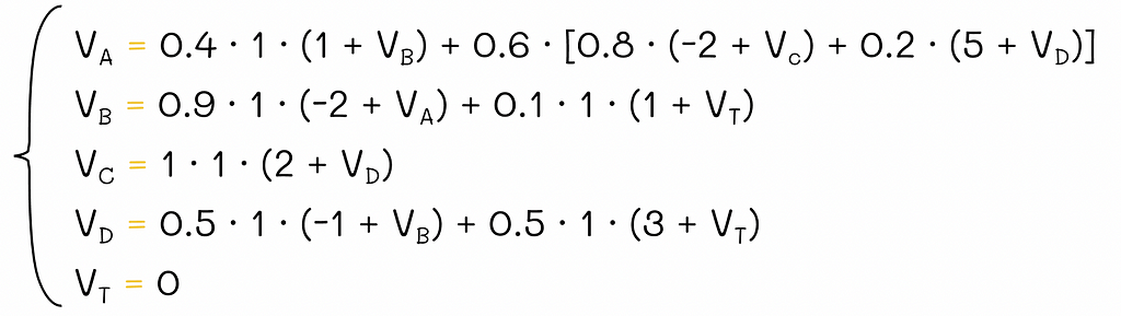
Since T is a terminal state, its v-value is always 0, so technically we only have to solve 4 equations.

Solving the analogous system for the Q-function would be harder because we would need to solve an equation for every pair (state, action).

Policy evaluation

Solving a linear system of equations in a straightforward manner, as it was shown in the example above, is a possible way to get real v-values. However, given the cubic algorithm complexity O(n³), where n = |S|, it is not optimal, especially when the number of states |S| is large. Instead, we can apply an iterative policy evaluation algorithm:

1. Randomly initialise v-values for all environment states (except for terminal states whose v-values must be equal to 0).
2. Iteratively update all non-terminal states by using the Bellman equation.
3. Repeat step 2 until the difference between previous and current v-values is too small (≤ θ).

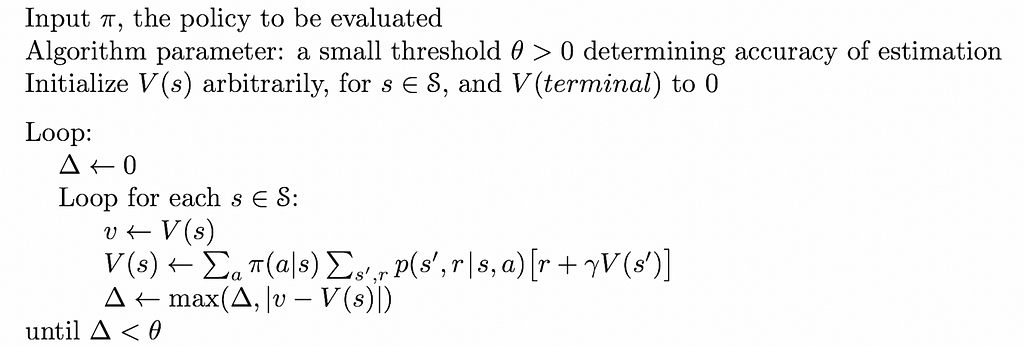
If the number of states |S| if finite, then it is possible to prove mathematically that iterative estimations obtained by the policy evaluation algorithm under a given policy π ultimately converge to real v-values!

A single update of the v-value of a state s ∈ S is called an expected update. The logic behind this name is that the update procedure considers rewards of all possible successive states of s, not just a single one.

A whole iteration of updates for all states is called a sweep.

Note. The analogous iterative algorithm can be applied to the calculation of Q-functions as well.

To realize how amazing this algorithm is, let us highlight it once again:

Policy evaluation allows iteratively finding the V-function under a given policy π.

Update variations

The update equation in the policy evaluation algorithm can be implemented in two ways:

• By using two arrays: new values are computed sequentially from unchanged old values stored in two separate arrays.
• By using one array: computed values are overwritten immediately. As a result, later updates during the same iteration use the overwritten new values.

In practice, overwriting v-values is a preferable way to perform updates because the new information is used as soon as it becomes available for other updates, in comparison to the two array method. As a consequence, v-values tend to converge faster.

The algorithm does not impose rules on the order of variables that should be updated during every iteration, however the order can have a large influence on the convergence rate.

Example

Description

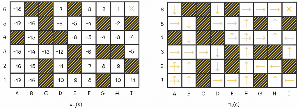
To further understand how the policy evaluation algorithm works in practice, let us have a look at the example 4.1 from the Sutton’s and Barto’s book. We are given an environment in the form of the 4 x 4 grid where at every step the agent equiprobably (p = 0.25) makes a single step in one of the four directions (up, right, down, left).

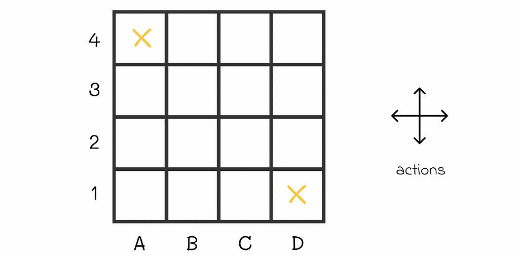
If an agent is located at the edge of the maze and chooses to go into the direction of a wall around the maze, then its position stays the same. For example, if the agent is located at D3 and chooses to go to the right, then it will stay at D3 at the next state.

Every move to any cell results in R = -1 reward except for two terminal states located at A4 and D1 whose rewards are R = 0. The ultimate goal is to calculate V-function for the given equiprobable policy.

Algorithm

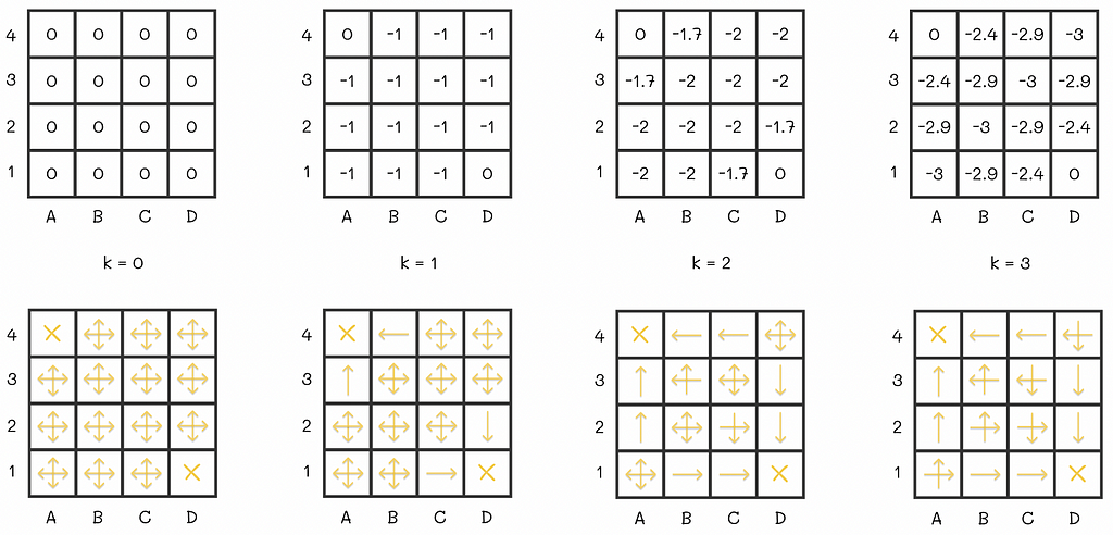
Let us initialize all V-values to 0. Then we will run several iterations of the policy evaluation algorithm:

At some point, there will be no changes between v-values on consecutive iterations. That means that the algorithm has converged to the real V-values. For the maze, the V-function under the equiprobable policy is shown at the right of the last diagram row.

Interpretation

Let us say an agent acting according to the random policy starts from the cell C2 whose expected reward is -18. By the V-function definition, -18 is the total cumulative reward the agent receives by the end of the episode. Since every move in the maze adds -1 to the reward, we can interpret the v-value of 18 as the expected number of steps the agent will have to make until it gets to the terminal state.

Policy improvement

At first sight, it might sound surprising but V- and Q- functions can be used to find optimal policies. To understand this, let us refer to the maze example where we have calculated the V-function for a starting random policy.

For instance, let us take the cell B3. Given our random policy, the agent can go in 4 directions with equal probabilities from that state. The possible expected rewards it can receive are -14, -20, -20 and -14. Let us suppose that we had an option to modify the policy for that state. To maximize the expected reward, would not it be logical to always go next to either A3 or B4 from B3, i.e. in the cell with the maximum expected reward in the neighbourhood (-14 in our case)?

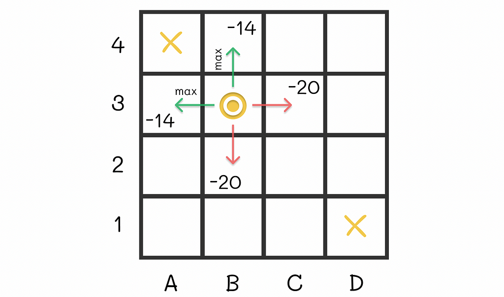
This idea makes sense because being located at A3 or B4 gives the agent a possibility to finish the maze in just one step. As a result, we can include that transition rule for B3 to derive a new policy. Nevertheless, is it always optimal to make such transitions to maximize the expected reward?

Indeed, transitioning greedily to the state with an action whose combination of expected reward is maximal among other possible next states, leads to a better policy.

To continue our example, let us perform the same procedure for all maze states:

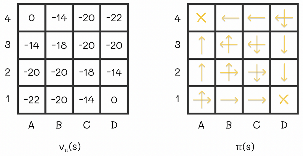
As a consequence, we have derived a new policy that is better than the old one. By the way, our findings can be generalized for other problems as well by the policy improvement theorem which plays a crucial role in reinforcement learning.

Policy improvement theorem

Formulation

The formulation from the Sutton’s and Barto’s book concisely describes the theorem:

Let π and π’ be any pair of deterministic policies such that, for all s ∈ S,

Then the policy π’ must be as good as, or better than, π. That is, it must obtain greater or equal expected return from all states s ∈ S:

Logic

To understand the theorem’s formulation, let us assume that we have access to the V- and Q-functions of a given environment evaluated under a policy π. For that environment, we will create another policy π’. This policy will be absolutely the same as π with the only difference that for every state it will choose actions that result in either the same or greater rewards. Then the theorem guarantees that the V-function under policy π’ will be better than the one for the policy π.

With the policy improvement theorem, we can always derive better policies by greedily choosing actions of the current policy that lead to maximum rewards for every state.

Policy iteration

Given any starting policy π, we can compute its V-function. This V-function can be used to improve the policy to π’. With this policy π’, we can calculate its V’-function. This procedure can be repeated multiple times to iteratively produce better policies and value functions.

In the limit, for a finite number of states, this algorithm, called policy iteration, converges to the optimal policy and the optimal value function.

If we applied the policy iteration algorithm to the maze example, then the optimal V-function and policy would look like this:

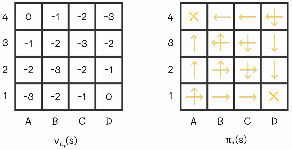
In these settings, with the obtained optimal V-function, we can easily estimate the number of steps required to get to the terminal state, according to the optimal strategy.

What is so interesting about this example is the fact that we would only need two policy iterations to obtain these values from scratch (we can notice that the optimal policy from the image is exactly the same as it was before when we had greedily updated it to the respective V-function). In some situations, the policy iteration algorithm requires only few iterations to converge.

Value iteration

Though the original policy iteration algorithm can be used to find optimal policies, it can be slow, mainly because of multiple sweeps performed during policy evaluation steps. Moreover, the full convergence process to the exact V-function might require a lot sweeps.

In addition, sometimes it is not necessary to get exact v-values to yield a better policy. The previous example demonstrates it perfectly: instead of performing multiple sweeps, we could have done only k = 3 sweeps and then built a policy based on the obtained approximation of the V-function. This policy would have been exactly the same as the one we have computed after V-function convergence.

In general, is it possible to stop the policy evaluation algorithm at some point? It turns out that yes! Furthermore, only a single sweep can be performed during every policy evaluation step and the result will still converge to the optimal policy. The described algorithm is called value iteration.

We are not going to study the proof of this algorithm. Nevertheless, we can notice that policy evaluation and policy improvement are two very similar processes to each other: both of them use the Bellman equation except for the fact that policy improvement takes the max operation to yield a better action.

By iteratively performing a single sweep of policy evaluation and a single sweep of policy improvement, we can converge faster to the optimum. In reality, we can stop the algorithm once the difference between successive V-functions becomes insignificant.

Asynchronous value iteration

In some situations, performing just a single sweep during every step of value iteration can be problematic, especially when the number of states |S| is large. To overcome this, asynchronous versions of the algorithm can be used: instead of systematically performing updates of all states during the whole sweep, only a subset of state values is updated in-place in whatever order. Moreover, some states can be updated multiple times before other states are updated.

However, at some point, all of the states will have to be updated, to make it possible for the algorithm to converge. According to the theory, all of the states must be updated in total an infinite number of times to achieve convergence but in practice this aspect is usually omitted since we are not always interested in getting 100% optimal policy.

There exist different implementations of asynchronous value iteration. In real problems, they make it possible to efficiently trade off between the algorithm’s speed and accuracy.

One of the the simplest asynchronous versions is to update only a single state during the policy evaluation.

Generalized policy iteration

We have looked at the policy iteration algorithm. Its idea can be used to refer to a broader term in reinforcement learning called generalized policy iteration (GPI).

The GPI consists of finding the optimal policy through independent alternation between policy evaluation and policy improvement processes.

Almost all of the reinforcement learning algorithms can be referred to as GPI.

Sutton and Barto provide a simplified geometric figure that intuitively explains how GPI works. Let us imagine a 2D plane where every point represents a combination of a value function and a policy. Then we will draw two lines:

• The first line will contain points corresponding to different V-functions of an environment.
• The second line will represent a set of greedy policies in relation to respective V-functions.

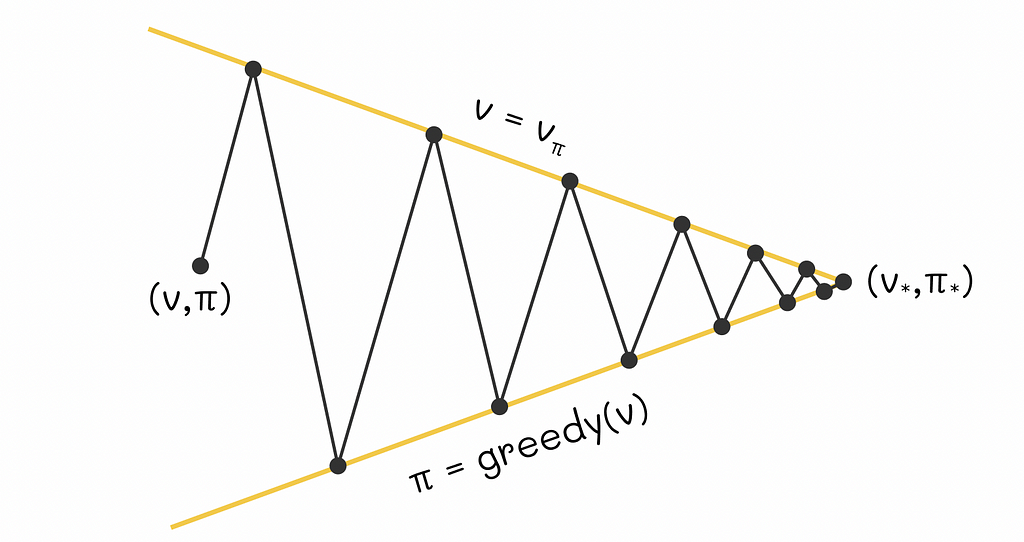
Every time when we calculate a greedy policy for the current V-function, we move closer to the policy line while moving away from the V-function line. That is logical because for the new computed policy, the previous V-function no longer applies. On the other hand, every time we perform policy evaluation, we move towards the projection of a point on the V-function line and thus we move further from the policy line: for the new estimated V-function, the current policy is no longer optimal. The whole process is repeated again.

As these two processes alternate between each other, both current V-function and policy gradually improve and at some moment in time they must reach a point of optimality that will represent an intersection between the V-function and policy lines.

Conclusion

In this article, we have gone through the main ideas behind policy evaluation and policy improvement. The beauty of these two algorithms is their ability to interact with each other to reach the optimal state. This approach only works in perfect environments where the agent’s probability transitions are given for all states and actions. Despite this constraint, many other reinforcement learning algorithms use the GPI method as a fundamental building block for finding optimal policies.

For environments with numerous states, several heuristics can be applied to accelerate the convergence speed one of which includes asynchronous updates during the policy evaluation step. Since the majority of reinforcement algorithms require a lot of computational resources, this technique becomes very useful and allows efficiently trading accuracy for gains in speed.

Resources

• Reinforcement Learning. An Introduction. Second Edition | Richard S. Sutton and Andrew G. Barto

All images unless otherwise noted are by the author.

---

Reinforcement Learning, Part 2: Policy Evaluation and Improvement was originally published in Towards Data Science on Medium, where people are continuing the conversation by highlighting and responding to this story.

A step-by-step guide to linking your AI agent with a SQL database — Part 2 of the series

Imagine streamlining your entire business management through a single, user-friendly interface on your phone. While juggling multiple apps is common practice, the future lies in consolidating all your interactions into one chat-based platform, powered by the capabilities of Large Language Models (LLMs).

For small businesses, this approach offers significant advantages. By centralizing data management tasks within a unified chat interface, owners can save time, reduce complexity, and minimize reliance on disparate software tools. The result is a more efficient allocation of resources, allowing a greater focus on core business growth activities.

However, the potential extends beyond just small businesses. The concepts and techniques detailed in this tutorial are adaptable to personal use cases as well. From managing to-do lists and tracking expenses to organizing collections, a chat-based interface provides an intuitive and efficient way to interact with your data.

This article is the second installment in a series that guides you through the process of developing such a software project, from initial concept to practical implementation. Building upon the components introduced in the previous article, we will establish the foundational elements of our application, including:

• Setting up the database schema
• Defining core application functionality
• Structuring the project repository
• Creating Tools capable of interacting with multiple SQL database tables using natural language commands

By the end of this tutorial, you will have a clear understanding of how to architect a chat-based interface that leverages LLMs to simplify data management tasks. Whether you’re a small business owner looking to streamline operations or an individual seeking to optimize personal organization, the principles covered here will provide a solid starting point for your own projects.

Let’s begin by briefly recapping the key takeaways from the previous article to set the context for our current objectives.

Recap

In the first part of this series, we built a prototype agent workflow capable of interacting with tool objects. Our goal was to reduce hallucination in tool arguments generated by the underlying language model, in our case gpt-3.5-turbo.

To achieve this, we implemented two key changes:

1. Removed required parameters in the tool schema
2. Added a parameter validation step before executing the desired function

By setting all tool parameters to optional and manually checking for missing parameters, we eliminated the urge for the Agent/LLM to hallucinate missing values.

The key objects introduced in the previous article were:

• OpenAiAgent: The main agent workflow class
• Tool: A class representing a tool the agent can use
• ToolResult and StepResult: Classes for encapsulating tool execution results

These components formed the foundation of our agent system, allowing it to process user requests, select appropriate tools, and generate responses.

If you’d like a more detailed explanation or want to know the reasoning behind specific design choices, feel free to check out the previous article: Leverage OpenAI Tool Calling: Building a Reliable AI Agent from Scratch

With this recap in mind, let’s dive into the next phase of our project — integrating database functionality to store and manage business data.

Why Chat Interface for Small Business Data Management

Small businesses often face unique challenges when it comes to data maintenance. Like larger corporations, they need to regularly update and maintain various types of data, such as accounting records, time tracking, invoices, and more. However, the complexity and costs associated with modern ERP (Enterprise Resource Planning) systems can be prohibitive for small businesses. As a result, many resort to using a series of Excel spreadsheets to capture and maintain essential data.

The problem with this approach is that small business owners, who are rarely dedicated solely to administrative tasks, cannot afford to invest significant time and effort into complex administration and control processes. The key is to define lean processes and update data as it arises, minimizing the overhead of data management.

By leveraging the power of Large Language Models and creating a chat interface, we aim to simplify and streamline data management for small businesses. The chatbot will act as a unified interface, allowing users to input data, retrieve information, and perform various tasks using natural language commands. This eliminates the need for navigating multiple spreadsheets or developing complex web applications with multiple forms and dashboards.

Throughout this series, we will gradually enhance the chatbot’s capabilities, adding features such as role-based access control, advanced querying and evaluation, multimodal support, and integration with popular communication platforms like WhatsApp. By the end of the series, you will have a powerful and flexible tool that can adapt to your specific needs, whether you’re running a small business or simply looking to organize your personal life more efficiently.

Let’s get started!

1. Project Structure

To ensure a well-organized and maintainable project, we’ve structured our repository to encapsulate different functionalities and components systematically. Here’s an overview of the repository structure:

project-root/
│
├── database/
│ ├── db.py # Database connection and setup
│ ├── models.py # Database models/schemas
| └── utils.py # Database utilities
│
├── tools/
│ ├── base.py # Base class for tools
│ ├── add.py # Tool for adding data to the database
│ ├── query.py # Tool for querying data from the database
| └── utils.py # Tool utilities
│
├── agents/
│ ├── base.py # Main AI agent logic
│ ├── routing.py # Specialized agent for routing tasks
│ ├── task.py # Tool wrapper for OpenAI subagents
| └── utils.py # agent utilities
│
└── utils.py # Utility functions and classes

This structure allows for a clear separation of concerns, making it easier to develop, maintain, and scale our application.

2. Set up Database

Choosing the right database and ORM (Object-Relational Mapping) library is crucial for our application. For this project, we’ve selected the following frameworks:

• SQLAlchemy: A powerful SQL toolkit and Object-Relational Mapping (ORM) library for Python. It provides a set of tools for interacting with databases using Python objects and classes.
• SQLModel: A library that builds on top of SQLAlchemy and Pydantic, offering a simple and intuitive way to define database models and perform database operations.

By leveraging SQLModel, we can seamlessly integrate with Pydantic and SQLAlchemy, enabling efficient data validation and database operations while eliminating the risk of SQL injection attacks. Moreover, SQLModel allows us to easily build upon our previously designed Tool class, which uses Pydantic models for creating a tool schema.

To ensure the security and robustness of our application, we implement the following measures:

1. Role-based access control: Executable operations are bound to user roles, ensuring that users can only perform actions they are authorized to do. This adds an extra layer of security and prevents unauthorized access to sensitive data.
2. Prevention of SQL injection attacks: By utilizing ChatGPT’s natural language understanding capabilities, we can validate and sanitize user inputs, mitigating the risk of SQL injection vulnerabilities. SQLModel’s integration with Pydantic helps us enforce strict data validation rules.

With our tech stack decided, let’s dive into setting up the database and defining our models.

2.1 Database Models

To begin building our prototype application, we’ll define the essential database tables and their corresponding SQLModel definitions. For this tutorial, we’ll focus on three core tables:

• Expense
• Revenue
• Customer

These tables will serve as the foundation for our application, allowing us to demonstrate the key functionalities and interactions.

Create a new file named models.py in the database directory and define the tables using SQLModel:

# databasemodels.py
from typing import Optional  
  
from pydantic import BeforeValidator, model_validator  
from sqlmodel import SQLModel, Field  
from datetime import time, datetime  
from typing_extensions import Annotated 

def validate_date(v):  
    if isinstance(v, datetime):  
        return v  
  
    for f in ["%Y-%m-%d", "%Y-%m-%d %H:%M:%S"]:  
        try:  
            return datetime.strptime(v, f)  
        except ValueError:  
            pass  
  
    raise ValueError("Invalid date format")  
  
  
def numeric_validator(v):  
    if isinstance(v, int):  
        return float(v)  
    elif isinstance(v, float):  
        return v  
    raise ValueError("Value must be a number")  
  
  
DateFormat = Annotated[datetime, BeforeValidator(validate_date)]  
Numeric = Annotated[float, BeforeValidator(numeric_validator)]
  
class Customer(SQLModel, table=True):  
    id: Optional[int] = Field(primary_key=True, default=None)
    company: str
    first_name: str  
    last_name: str  
    phone: str  
    address: str  
    city: str  
    zip: str  
    country: str  
  
  
class Revenue(SQLModel, table=True):  
    id: Optional[int] = Field(primary_key=True, default=None)  
    description: str  
    net_amount: Numeric  
    gross_amount: Numeric  
    tax_rate: Numeric  
    date: DateFormat  
  
  
class Expense(SQLModel, table=True):  
    id: Optional[int] = Field(primary_key=True, default=None)  
    description: str  
    net_amount: Numeric = Field(description="The net amount of the expense")  
    gross_amount: Numeric  
    tax_rate: Numeric  
    date: DateFormat

In addition to the standard SQLModel fields, we’ve defined three custom type annotations: DateFormat, TimeFormat, and Numeric. These annotations leverage Pydantic’s BeforeValidator to ensure that the input data is correctly formatted before being stored in the database. The validate_date function handles the conversion of string input to the appropriate datetime. This approach allows us to accept a variety of date formats from the Large Language Model, reducing the need for strict format enforcement in the prompts.

2.2 Database Engine

With our models defined, we need a script to set up the database engine and create the corresponding tables. Let’s create a db.py file in the database directory to handle this:

# database/db.py
from database.models import *  
from sqlmodel import SQLModel, create_engine  
import os  
  
  
# local stored database  
DATABASE_URL = "sqlite:///app.db"  
  
engine = create_engine(DATABASE_URL, echo=True) 
  
  
def create_db_and_tables():  
    SQLModel.metadata.create_all(engine)  
  
  
create_db_and_tables()

In this script, we import our models and the necessary SQLModel components. We define the DATABASE_URL to point to a local SQLite database file named app.db. We create an engine using create_engine from SQLModel, passing in the DATABASE_URL. The echo=True parameter enables verbose output for debugging purposes.

The create_db_and_tables function uses SQLModel.metadata.create_all to generate the corresponding tables in the database based on our defined models. Finally, we call this function to ensure the database and tables are created when the script is run.

With our database setup complete, we can now focus on updating our Tool class to work seamlessly with SQLModel and enhance our tool schema conversion process.

3. Tool Class

In this section, we’ll discuss the updates made to the Tool class to handle SQLModel instances and improve the validation process. For a more detailed explanation of the Tool class, visit my previous article.

First, we’ve added Type[SQLModel] as a possible type for the model field using the Union type hint. This allows the Tool class to accept both Pydantic’s BaseModel and SQLModel’s SQLModel as valid model types.

Next, we’ve introduced a new attribute called exclude_keys of type list[str] with a default value of [“id”]. The purpose of this attribute is to specify which keys should be excluded from the validation process and the OpenAI tool schema generation. In this case the default excluded key is id since for data entry creation with SqlModel the id is automatically generated during ingestion.

On top of that we introduced parse_model boolean attribute to our Tool class. Where we can basically decided if the tool function is called with our pydantic/SQLModel or with keyword arguments.

In the validate_input() method, we’ve added a check to ensure that the keys specified in exclude_keys are not considered as missing keys during the validation process. This is particularly useful for fields like id, which are automatically generated by SQLModel and should not be required in the input.

Similarly, in the openai_tool_schema property, we’ve added a loop to remove the excluded keys from the generated schema. This ensures that the excluded keys are not included in the schema sent to the OpenAI API. For recap we use the openai_tool_schema property to remove required arguments from our tool schema. This is done to elimenate hallucination by our language model.

Moreover, we changed the import from from pydantic.v1 import BaseModel to from pydantic import BaseModel. Since SQLModel is based on Pydantic v2, we want to be consistent and use Pydantic v2 at this point.

Here’s the updated code for the Tool class:

# tools/base.py
from typing import Type, Callable, Union

from tools.convert import convert_to_openai_tool
from pydantic import BaseModel, ConfigDict
from sqlmodel import SQLModel


class ToolResult(BaseModel):
    content: str
    success: bool


class Tool(BaseModel):
    name: str
    model: Union[Type[BaseModel], Type[SQLModel], None]
    function: Callable
    validate_missing: bool = True
    parse_model: bool = False
    exclude_keys: list[str] = ["id"]

    model_config = ConfigDict(arbitrary_types_allowed=True)

    def run(self, **kwargs) -> ToolResult:
        if self.validate_missing and model is not None:
            missing_values = self.validate_input(**kwargs)
            if missing_values:
                content = f"Missing values: {', '.join(missing_values)}"
                return ToolResult(content=content, success=False)

        if self.parse_model:
            if hasattr(self.model, "model_validate"):
                input_ = self.model.model_validate(kwargs)
            else:
                input_ = self.model(**kwargs)
            result = self.function(input_)

        else:
            result = self.function(**kwargs)
        return ToolResult(content=str(result), success=True)

    def validate_input(self, **kwargs):
        if not self.validate_missing or not self.model:
            return []
        model_keys = set(self.model.__annotations__.keys()) - set(self.exclude_keys)
        input_keys = set(kwargs.keys())
        missing_values = model_keys - input_keys
        return list(missing_values)

    @property
    def openai_tool_schema(self):
        schema = convert_to_openai_tool(self.model)
        # set function name
        schema["function"]["name"] = self.name

        # remove required field
        if schema["function"]["parameters"].get("required"):
            del schema["function"]["parameters"]["required"]
        # remove exclude keys
        if self.exclude_keys:
            for key in self.exclude_keys:
                if key in schema["function"]["parameters"]["properties"]:
                    del schema["function"]["parameters"]["properties"][key]
        return schema

These updates to the Tool class provide more flexibility and control over the validation process and schema generation when working with SQLModel instances.

3.1 Custom Tool Schema Conversion

In our Tool class, we create a schema from a Pydantic model using the convert_to_openai_tool function from Langchain. However, this function is based on Pydantic v1, while SQLModel uses Pydantic v2. To make the conversion function compatible, we need to adapt it. Let’s create a new script called convert.py:

# tools/convert.py
from langchain_core.utils.function_calling import _rm_titles
from typing import Type, Optional
from langchain_core.utils.json_schema import dereference_refs
from pydantic import BaseModel

def convert_to_openai_tool(
        model: Type[BaseModel],
        *,
        name: Optional[str] = None,
        description: Optional[str] = None,
) -> dict:
    """Converts a Pydantic model to a function description for the OpenAI API."""
    function = convert_pydantic_to_openai_function(
        model, name=name, description=description
    )
    return {"type": "function", "function": function}

def convert_pydantic_to_openai_function(
        model: Type[BaseModel],
        *,
        name: Optional[str] = None,
        description: Optional[str] = None,
        rm_titles: bool = True,
) -> dict:
    """Converts a Pydantic model to a function description for the OpenAI API."""

    model_schema = model.model_json_schema() if hasattr(model, "model_json_schema") else model.schema()
    
    schema = dereference_refs(model_schema)
    schema.pop("definitions", None)
    title = schema.pop("title", "")
    default_description = schema.pop("description", "")
    return {
        "name": name or title,
        "description": description or default_description,
        "parameters": _rm_titles(schema) if rm_titles else schema,
    }

This adapted conversion function handles the differences between Pydantic v1 and v2, ensuring that our Tool class can generate compatible schemas for the OpenAI API.

Next, update the import statement in tools/base.py to use the new convert_to_openai_tool function:

# tools/base.py
from typing import Type, Callable, Union

from tools.convert import convert_to_openai_tool
from pydantic import BaseModel
from sqlmodel import SQLModel
#...rest of the code ...

With these changes in place, our Tool class can now handle SQLModel instances and generate schemas that are compatible with the OpenAI API.

Note: If you encounter dependency issues, you may consider removing the Langchain dependency entirely and including the _rm_titles and dereference_refs functions directly in the convert.py file.

By adapting the tool schema conversion process, we’ve ensured that our application can seamlessly work with SQLModel and Pydantic v2, enabling us to leverage the benefits of these libraries while maintaining compatibility with the OpenAI API.

4. Defining SQL Tools

In this section, we will create functions and tools to interact with our database tables using SQL.

4.1 Add Data Tool

First, let’s define a generic function add_row_to_table that takes a SQLModel instance and adds it to the corresponding table:

# tools/add.py
from sqlmodel import SQLModel, Session, select

def add_row_to_table(model_instance: SQLModel):  
    with Session(engine) as session:  
        session.add(model_instance)  
        session.commit()  
        session.refresh(model_instance)  
    return f"Successfully added {model_instance} to the table"

Next, we’ll create a model-specific function add_expense_to_table that takes input arguments for an Expense entry and adds it to the table:

# tools/add.py
# ...
def add_expense_to_table(**kwargs):
    model_instance = Expense.model_validate(kwargs)
    return add_row_to_table(model_instance)

In add_expense_to_table, we use the model_validate() method to trigger the execution of the previously defined BeforeValidator and ensure data validation.

To avoid writing separate functions for each table or SQLModel, we can dynamically generate the functions:

# example usage

def add_entry_to_table(sql_model: Type[SQLModel]):  
    # return a Callable that takes a SQLModel instance and adds it to the table  
    return lambda **data: add_row_to_table(model_instance=sql_model.model_validate(data))
    
add_expense_to_table = add_entry_to_table(Expense)

This approach produces the same result and can be used to dynamically generate functions for all other models.

With these functions in place, we can create tools using our Tool class to add entries to our database tables via the OpenAIAgent:

add_expense_tool = Tool(
 name="add_expense_tool",
 description="useful for adding expenses to database",
 function=add_entry_to_table(Expense),
 model=Expense,
 validate_missing=True
)

add_revenue_tool = Tool(
 name="add_revenue_tool",
 description="useful for adding revenue to database",
 function=add_entry_to_table(Revenue),
 model=Revenue,
 validate_missing=True
)

4.2 Query Tool

While we need to create an add_xxx_tool for each table due to varying input schemas, we only need one query tool for querying all tables. To eliminate the risk of SQL injection, we will use the SQL sanitization provided by SQLAlchemy and SQLModel. This means we will query the database through standard Python classes and objects instead of parsing SQL statements directly.

For the queries we want to perform on our tables, we will need the following logic:

1. select statement -> SELECT * FROM table_name Arguments: columns, table_name
2. where statement -> WHERE column_name = value
   Arguments: column, operator, value

In SQLModel, this corresponds to the following sanitized code when we want to find all expenses for coffee in the Expense table:

result = database.execute(
  select(Expense).where(Expense.description == "Coffee")
)

To abstract this into a pydantic model:

# tools/query.py
from typing import Union, Literal
from pydantic import BaseModel

class WhereStatement(BaseModel):  
    column: str  
    operator: Literal["eq", "gt", "lt", "gte", "lte", "ne", "ct"]  
    value: str  
  
class QueryConfig(BaseModel):  
    table_name: str  
    columns: list[str]  
    where: list[Union[WhereStatement, None]]

The QueryConfig model allows us to set a table_name, columns, and where statements. The where property accepts a list of WhereStatement models or an empty list (when we want to return all values with no further filtering). A WhereStatement is a submodel defining a column, operator, and value. The Literal type is used to restrict the allowed operators to a predefined set.

Next, we define a function that executes a query based on the QueryConfig:

# tools/query.py
# ...
from database.models import Expense, Revenue, Customer

TABLES = {
    "expense": Expense,
    "revenue": Revenue,
    "customer": Customer
}



def query_data_function(**kwargs) -> ToolResult:  
    """Query the database via natural language."""
    query_config = QueryConfig.model_validate(kwargs)
    
    if query_config.table_name not in TABLES:  
        return ToolResult(content=f"Table name {query_config.table_name} not found in database models", success=False)  
  
    sql_model = TABLES[query_config.table_name]  
  
    # query_config = validate_query_config(query_config, sql_model)  
    data = sql_query_from_config(query_config, sql_model)  
  
    return ToolResult(content=f"Query results: {data}", success=True)  
    
  
def sql_query_from_config(  
        query_config: QueryConfig,  
        sql_model: Type[SQLModel]):  
  
    with Session(engine) as session:  
        selection = []  
        for column in query_config.select_columns:  
            if column not in sql_model.__annotations__:  
                return f"Column {column} not found in model {sql_model.__name__}"  
            selection.append(getattr(sql_model, column))  
        
        statement = select(*selection)  
        wheres = query_config.where  
        if wheres:  
            for where in wheres:  
  
                if where.column not in sql_model.__annotations__:  # noqa  
                    return (f"Column {where['column']} not found "
                       "in model {sql_model.__name__}")
  
                elif where.operator == "eq":  
                    statement = statement.where(
                     getattr(sql_model, where.column) == where.value)  
                elif where.operator == "gt":  
                    statement = statement.where(
                     getattr(sql_model, where.column) > where.value)  
                elif where.operator == "lt":  
                    statement = statement.where(
                     getattr(sql_model, where.column) < where.value)  
                elif where.operator == "gte":  
                    statement = statement.where(
                     getattr(sql_model, where.column) >= where.value)  
                elif where.operator == "lte":  
                    statement = statement.where(
                     getattr(sql_model, where.column) <= where.value)  
                elif where.operator == "ne":  
                    statement = statement.where(
                     getattr(sql_model, where.column) != where.value)  
                elif where.operator == "ct":  
                    statement = statement.where(
                     getattr(sql_model, where.column).contains(where.value))  
  
        result = session.exec(statement)  
        data = result.all()  
        try:  
            data = [repr(d) for d in data]  
        except:  
            pass  
    return data

The query_data_function serves as a high-level abstraction for selecting our table model from the TABLES dictionary, while sql_query_from_config is the underlying function for executing the QueryConfig on a table (SQLModel).

In `QueryConfig` you can choose to also define table_names as Literal type, where you hard code the available table names into it. You can even dynamically define the Literal using our TABLES dictionary. By doing so you can reduce false arguments for table_name. For now I have choosen to not use an enum object, because I will provide the agent prompt with context about the currently available tables and there underling ORM schema. I plan to add a tool for our future agent to create new tables on it’s own.While I can dynamically change the agent’s prompt, it won’t be straightforward to change the enum object within `QueryConfig` on our running server.

Finally, we can define our query tool:

query_data_tool = Tool(  
    name="query_data_tool",  
    description = "useful to perform queries on a database table",
    model=QueryConfig,  
    function=query_data_function, 
)

With these tools in place, our OpenAIAgent is now capable of adding and querying data in our database tables using natural language commands.

5. Configure Agent

To enable successful tool usage for our previously defined tools, the Agent from the previous article will need more context information, especially for using the query tool. The Agent prompt will need to include information about available tables and their schemas. Since we only use two tables at this point, we can include the ORM schema and table names in the system prompt or user prompt. Both options might work well, but I prefer to include variable information like this in the user prompt. By doing so, we can create few-shot examples that demonstrate context-aware tool usage.

To make our Agent capable of handling variable context in the system prompt and user prompt, we can update our Agent class as follows:

import colorama  
from colorama import Fore  
from openai import OpenAI  
from pydantic import BaseModel  
from tools.base import Tool, ToolResult  
from agents.utils import parse_function_args, run_tool_from_response  
  
  
class StepResult(BaseModel):  
    event: str  
    content: str  
    success: bool  
  
  
SYSTEM_MESSAGE = """You are tasked with completing specific objectives and must report the outcomes. At your disposal, you have a variety of tools, each specialized in performing a distinct type of task.  
  
For successful task completion:  
Thought: Consider the task at hand and determine which tool is best suited based on its capabilities and the nature of the work. If you can complete the task or answer a question, soley by the information provided you can use the report_tool directly.  
  
Use the report_tool with an instruction detailing the results of your work or to answer a user question.  
If you encounter an issue and cannot complete the task:  
  
Use the report_tool to communicate the challenge or reason for the task's incompletion.  
You will receive feedback based on the outcomes of each tool's task execution or explanations for any tasks that couldn't be completed. This feedback loop is crucial for addressing and resolving any issues by strategically deploying the available tools.  
  
Return only one tool call at a time.  
  
{context}  
"""


class OpenAIAgent:  
  
    def __init__(  
            self,  
            tools: list[Tool],  
            client: OpenAI = OpenAI(),  
            system_message: str = SYSTEM_MESSAGE,  
            model_name: str = "gpt-3.5-turbo-0125",  
            max_steps: int = 5,  
            verbose: bool = True,  
            examples: list[dict] = None,  
            context: str = None,  
            user_context: str = None  
    ):  
        self.tools = tools  
        self.client = client  
        self.model_name = model_name  
        self.system_message = system_message  
        self.step_history = []  
        self.max_steps = max_steps  
        self.verbose = verbose  
        self.examples = examples or []  
        self.context = context or ""  
        self.user_context = user_context  
  
    def to_console(self, tag: str, message: str, color: str = "green"):  
        if self.verbose:  
            color_prefix = Fore.__dict__[color.upper()]  
            print(color_prefix + f"{tag}: {message}{colorama.Style.RESET_ALL}")  
  
    def run(self, user_input: str, context: str = None):  
  
        openai_tools = [tool.openai_tool_schema for tool in self.tools]  
        system_message = self.system_message.format(context=context)  
  
        if self.user_context:  
            context = f"{self.user_context}n{context}" if context else self.user_context  
  
        if context:  
            user_input = f"{context}n---nnUser Message: {user_input}"  
  
        self.to_console("START", f"Starting Agent with Input:n'''{user_input}'''")  
  
  
        self.step_history = [  
            {"role": "system", "content": system_message},  
            *self.examples,  
            {"role": "user", "content": user_input}  
        ]  
  
        step_result = None  
        i = 0  
  
        while i < self.max_steps:  
            step_result = self.run_step(self.step_history, openai_tools)  
            if step_result.event == "finish":  
                break  
            elif step_result.event == "error":  
                self.to_console(step_result.event, step_result.content, "red")  
            else:  
                self.to_console(step_result.event, step_result.content, "yellow")  
  
            i += 1  
  
        self.to_console("Final Result", step_result.content, "green")  
  
        return step_result.content  
  
    def run_step(self, messages: list[dict], tools):  
  
        # plan the next step  
        response = self.client.chat.completions.create(  
            model=self.model_name,  
            messages=messages,  
            tools=tools  
        )  
        # check for multiple tool calls  
        if response.choices[0].message.tool_calls and len(response.choices[0].message.tool_calls) > 1:  
            messages = [  
                *self.step_history,  
                {"role": "user", "content": "Error: Please return only one tool call at a time."}  
            ]  
            return self.run_step(messages, tools)  
  
        # add message to history  
        self.step_history.append(response.choices[0].message)  
        # check if tool call is present  
        if not response.choices[0].message.tool_calls:  
            msg = response.choices[0].message.content  
            step_result = StepResult(event="Error", content=f"No tool calls were returned.nMessage: {msg}", success=False)  
            return step_result  
  
        tool_name = response.choices[0].message.tool_calls[0].function.name  
        tool_kwargs = parse_function_args(response)  
  
        # execute the tool call  
        self.to_console("Tool Call", f"Name: {tool_name}nArgs: {tool_kwargs}", "magenta")  
        tool_result = run_tool_from_response(response, tools=self.tools)  
        tool_result_msg = self.tool_call_message(response, tool_result)  
        self.step_history.append(tool_result_msg)  
  
        if tool_name == "report_tool":  
            try:  
                step_result = StepResult(  
                    event="finish",  
                    content=tool_result.content,  
                    success=True  
                )  
            except:  
                print(tool_result)  
                raise ValueError("Report Tool failed to run.")  
  
            return step_result  
  
        elif tool_result.success:  
            step_result = StepResult(  
                event="tool_result",  
                content=tool_result.content,  
                success=True)  
        else:  
            step_result = StepResult(  
                event="error",  
                content=tool_result.content,  
                success=False  
            )  
  
        return step_result  
  
    def tool_call_message(self, response, tool_result: ToolResult):  
        tool_call = response.choices[0].message.tool_calls[0]  
        return {  
            "tool_call_id": tool_call.id,  
            "role": "tool",  
            "name": tool_call.function.name,  
            "content": tool_result.content,  
        }

The main changes compared to our previous version:

• We placed a “{context}” placeholder in the default system prompt.
• We added context and user_context as input arguments to __init__().
• We added context to the run() method.
• In run(), we add context to the user message if defined.
• We also added an examples attribute to __init__() that, if set, will be passed between the system and user messages in run().

Now we can define a system context and a user context while initializing our agent. Additionally, we can pass a user context when calling the run method. If context is passed to the run method, it will overwrite the user_context from initialization for that run.

5.1 Providing Context to the Agent

Before we can run our Agent, let’s define a function that generates context information. We want to automatically generate user_context, which we can then pass to the Agent’s run function as implemented above. To keep it simple, we want a single line for each table as context information that should include:

• Table name
• Column_name: <type>

After a few attempts with trial and error, the following function will do the job:

# utils.py
from typing import Type  
import types  
import typing  
  
import sqlalchemy  
from pydantic import BaseModel

def orm_model_to_string(input_model_cls: Type[BaseModel]):  
    """Get the ORM model string from the input model"""  
  
    def process_field(key, value):  
        if key.startswith("__"):  
            return None  
        if isinstance(value, typing._GenericAlias):  
            if value.__origin__ == sqlalchemy.orm.base.Mapped:  
                return None  
            if isinstance(value, typing._AnnotatedAlias):  # noqa  
                return key, value.__origin__  
            elif isinstance(value, typing._UnionGenericAlias) or isinstance(value, types.UnionType):  
                return key, value.__args__[0]  
        return key, value  
  
    fields = dict(filter(None, (process_field(k, v) for k, v in input_model_cls.__annotations__.items())))  
    return ", ".join([f"{k} = <{v.__name__}>" for k, v in fields.items()])

def generate_context(*table_models) -> str:
   context_str = "You can access the following tables in database:n"
   for table in table_models:
    context_str += f" - {table.__name__}: {orm_model_to_string(table)}n" 
   return context_str

If we pass Expense and Revenue to generate_context(), we should get the following context string:

We want the Agent to know the current date and day of the week, so we can reference the correct date. So let’s add some date parsing functions to our utils class:

# utils.py
from datetime import datetime

#... rest of utils.py ...

def weekday_by_date(date: datetime):
    days = ["Monday", "Tuesday", "Wednesday", "Thursday", "Friday", "Saturday", "Sunday"]
    return days[date.weekday()]


def date_to_string(date: datetime):
    return f"{weekday_by_date(date)} {parse_date(date)}"


def parse_date(date: datetime):
    return date.strftime("%Y-%m-%d")

Now let’s create the context for a query agent

# utils.py

# ...

def generate_query_context(*table_models) -> str:
    today = f"Today is {date_to_string(datetime.now())}"
    context_str = "You can access the following tables in database:n"
    for table in table_models:
        context_str += f" - {table.__name__}: {orm_model_to_string(table)}n" 
    return f"{today}n{context_str}"

from database.models import Expense, Revenue
print(generate_query_context(Expense, Revenue))

Today is Sunday 2024-04-21
You can access the following tables in database:
 - Expense: id = <int>, description = <str>, net_amount = <float>, gross_amount = <float>, tax_rate = <float>, date = <datetime>
 - Revenue: id = <int>, description = <str>, net_amount = <float>, gross_amount = <float>, tax_rate = <float>, date = <datetime>

5.2 Routing Agent

As we add more tools, the complexity of our setup may start to limit the usability of cheaper models like “gpt-3.5-turbo”. In the next article, we might consider switching to Anthropic Claude, since their newly released tool-use API feature seems promising, even for the more affordable HAIKU model, in handling multiple tools simultaneously. However, for now, we will continue using OpenAI’s GPT models.

When developing for personal use and before creating production-ready applications, I find it useful to optimize the workflow for smaller models, such as gpt-3.5-turbo in this case. This approach forces us to create a streamlined processing logic and prompting system. While we may not achieve 100% reliability without using the most powerful model, we will be able to catch flaws and identify unclear instructions. If your application works in 9 out of 10 cases with a smaller model, you will have a production-ready logic that will perform even better with a stronger model.

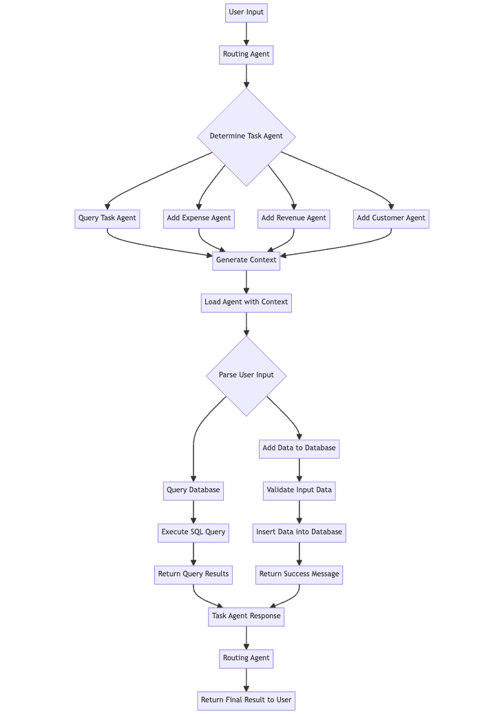
To make multi-tool handling reliable with gpt-3.5-turbo we will implement a routing agent whose sole purpose is to route the user query to the appropriate task agent. This allows us to separate execution logic and reduce complexity. Each agent will have a limited scope, enabling us to separate access roles and operations in the future. I have observed that even with gpt-4, there are instances where the agent does not know when its task is finished.

By introducing a routing agent, we can break down the problem into smaller, more manageable parts. The routing agent will be responsible for understanding the user’s intent and directing the query to the relevant task agent. This approach not only simplifies the individual agents’ responsibilities but also makes the system more modular and easier to maintain.

Furthermore, separating the execution logic and complexity will pave the way for implementing role-based access control in the future. Each task agent can be assigned specific permissions and access levels, ensuring that sensitive operations are only performed by authorized agents.

While the routing agent adds an extra step in the process, it ultimately leads to a more robust and scalable system. By optimizing for smaller models and focusing on clear, concise prompts, we can create a solid foundation that will perform even better when we switch to more powerful models like Claude Opus or GPT-4.

Let’s have a look on the implementation of the routing agent

# agents/routing.py
from openai import OpenAI
import colorama
from agents.task_agent import TaskAgent
from agents.utils import parse_function_args


SYSTEM_MESSAGE = """You are a helpful assistant.
Role: You are an AI Assistant designed to serve as the primary point of contact for users interacting through a chat interface. 
Your primary role is to understand users' requests related to database operations and route these requests to the appropriate tool.

Capabilities: 
You have access to a variety of tools designed for Create, Read operations on a set of predefined tables in a database. 

Tables:
{table_names}
"""

NOTES = """Important Notes:
Always confirm the completion of the requested operation with the user.
Maintain user privacy and data security throughout the interaction.
If a request is ambiguous or lacks specific details, ask follow-up questions to clarify the user's needs."""




class RoutingAgent:

    def __init__(
            self,
            tools: list[TaskAgent] = None,
            client: OpenAI = OpenAI(),
            system_message: str = SYSTEM_MESSAGE,
            model_name: str = "gpt-3.5-turbo-0125",
            max_steps: int = 5,
            verbose: bool = True,
            prompt_extra: dict = None,
            examples: list[dict] = None,
            context: str = None
    ):
        self.tools = tools or ROUTING_AGENTS
        self.client = client
        self.model_name = model_name
        self.system_message = system_message
        self.memory = []
        self.step_history = []
        self.max_steps = max_steps
        self.verbose = verbose
        self.prompt_extra = prompt_extra or PROMPT_EXTRA
        self.examples = self.load_examples(examples)
        self.context = context or ""

    def load_examples(self, examples: list[dict] = None):
        examples = examples or []
        for agent in self.tools:
            examples.extend(agent.routing_example)
        return examples

    def run(self, user_input: str, employee_id: int = None, **kwargs):
        context = create_routing_agent_context(employee_id)
        if context:
            user_input_with_context = f"{context}n---nnUser Message: {user_input}"
        else:
            user_input_with_context = user_input

        self.to_console("START", f"Starting Task Agent with Input:n'''{user_input_with_context}'''")
        partial_variables = {**self.prompt_extra, "context": context}
        system_message = self.system_message.format(**partial_variables)

        messages = [
            {"role": "system", "content": system_message},
            *self.examples,
            {"role": "user", "content": user_input}
        ]

        tools = [tool.openai_tool_schema for tool in self.tools]

        response = self.client.chat.completions.create(
            model=self.model_name,
            messages=messages,
            tools=tools
        )
        self.step_history.append(response.choices[0].message)
        self.to_console("RESPONSE", response.choices[0].message.content, color="blue")
        tool_kwargs = parse_function_args(response)
        tool_name = response.choices[0].message.tool_calls[0].function.name
        self.to_console("Tool Name", tool_name)
        self.to_console("Tool Args", tool_kwargs)

        agent = self.prepare_agent(tool_name, tool_kwargs)
        return agent.run(user_input)

    def prepare_agent(self, tool_name, tool_kwargs):
        for agent in self.tools:
            if agent.name == tool_name:
                input_kwargs = agent.arg_model.model_validate(tool_kwargs)
                return agent.load_agent(**input_kwargs.dict())
        raise ValueError(f"Agent {tool_name} not found")

    def to_console(self, tag: str, message: str, color: str = "green"):
        if self.verbose:
            color_prefix = colorama.Fore.__dict__[color.upper()]
            print(color_prefix + f"{tag}: {message}{colorama.Style.RESET_ALL}")

The biggest differences to our OpenAIAgent are:

• No open loop: we want the routing agent to route user’s queries to the appropriate agent. So instead of creating an open loop we select the desired agent via tool calling and pass the user query to it. The routing Agent should not do any other task or follow-up question.
• Agents as Tools: Instead of calling a tool the routing agent setup a subagent. So our previously defined OpenAIAgentis now a tool within our routing agent.

5.3 Agent as a Tool — Task Agent

To use our OpenAIAgentas a tool, we need to introduce some sort of tool class dedicated for Agents. We want to define a name and description for each agent and automate the initialization process. Therefore, we define our last class for this tutorial theTaskAgent.

The TaskAgent class serves similar functionality as the Tool class. We define a name a description and an input model which we call arg_model.

from typing import Type, Callable, Optional

from agents.base import OpenAIAgent
from tools.base import Tool
from tools.report_tool import report_tool
from pydantic import BaseModel, ConfigDict, Field

from tools.utils import convert_to_openai_tool


SYSTEM_MESSAGE = """You are tasked with completing specific objectives and must report the outcomes. At your disposal, you have a variety of tools, each specialized in performing a distinct type of task.

For successful task completion:
Thought: Consider the task at hand and determine which tool is best suited based on its capabilities and the nature of the work. 
If you can complete the task or answer a question, soley by the information provided you can use the report_tool directly.

Use the report_tool with an instruction detailing the results of your work or to answer a user question.
If you encounter an issue and cannot complete the task:

Use the report_tool to communicate the challenge or reason for the task's incompletion.
You will receive feedback based on the outcomes of each tool's task execution or explanations for any tasks that couldn't be completed. This feedback loop is crucial for addressing and resolving any issues by strategically deploying the available tools.

On error: If information are missing consider if you can deduce or calculate the missing information and repeat the tool call with more arguments.

Use the information provided by the user to deduct the correct tool arguments.
Before using a tool think about the arguments and explain each input argument used in the tool. 
Return only one tool call at a time! Explain your thoughts!
{context}
"""


class EmptyArgModel(BaseModel):
    pass


class TaskAgent(BaseModel):
    name: str
    description: str
    arg_model: Type[BaseModel] = EmptyArgModel

    create_context: Callable = None
    create_user_context: Callable = None
    tool_loader: Callable = None

    system_message: str = SYSTEM_MESSAGE
    tools: list[Tool]
    examples: list[dict] = None
    routing_example: list[dict] = Field(default_factory=list)

    model_config = ConfigDict(arbitrary_types_allowed=True)

    def load_agent(self, **kwargs) -> OpenAIAgent:

        input_kwargs = self.arg_model(**kwargs)
        kwargs = input_kwargs.dict()

        context = self.create_context(**kwargs) if self.create_context else None
        user_context = self.create_user_context(**kwargs) if self.create_user_context else None

        if self.tool_loader:
            self.tools.extend(self.tool_loader(**kwargs))

        if report_tool not in self.tools:
            self.tools.append(report_tool)

        return OpenAIAgent(
            tools=self.tools,
            context=context,
            user_context=user_context,
            system_message=self.system_message,
            examples=self.examples,
        )

    @property
    def openai_tool_schema(self):
        return convert_to_openai_tool(self.arg_model, name=self.name, description=self.description)

Additionally, we added all relevant attributes to our TaskAgent class, which we need for an underlying specialized OpenAIAgent :

• create_context / create_user_context: Here we can pass a function to create the context or user context like in section 5.1
• tool_loader is another callable function which we may need for setting up the underlying agent. As in our dynamic tool building previously explained, we may need tools that are dynamically built based on the user input/routing agent input.
• system_message is the agent’s system prompt. In our example, it will be the default system prompt for every agent, but it can be an optimized version for each specialized agent.
• tools: Predefined tools the agent should use.
• examples: Examples to include in subagent’s message history
• routing_example: Examples to include in routing agent’s message history

Moreover, we have an emty BaseModel called EmptyArgModel which is default arg_model in our TaskAgent

Let’s see if it all plays together!

Run Agent

Now, it’s time to test if our routing and subagents work well together. As we introduced examples as a paremeter we can use several test runs to inspect major flaws in the execution and define example usage for each sub agent.

Let’s define our subagents first:

from database.models import Expense, Revenue, Customer
from agents.task import TaskAgent
from utils import generate_query_context

from tools.base import Tool
from tools.query import query_data_tool
from tools.add import add_entry_to_table


query_task_agent = TaskAgent(
    name="query_agent",
    description="An agent that can perform queries on multiple data sources",
    create_user_context=lambda: generate_query_context(Expense, Revenue, Customer),
    tools=[query_data_tool]
)

add_expense_agent = TaskAgent(
    name="add_expense_agent",
    description="An agent that can add an expense to the database",
    create_user_context=lambda: generate_query_context(Expense) + "nRemarks: The tax rate is 0.19. The user provide the net amount you need to calculate the gross amount.",
    tools=[
        Tool(
            name="add_expense",
            description="Add an expense to the database",
            function=add_entry_to_table(Expense),
            model=Expense
        )
    ]
)

add_revenue_agent = TaskAgent(
    name="add_revenue_agent",
    description="An agent that can add a revenue entry to the database",
    create_user_context=lambda: generate_query_context(Revenue) + "nRemarks: The tax rate is 0.19. The user provide the gross_amount you should use the tax rate to calculate the net_amount.",
    tools=[
        Tool(
            name="add_revenue",
            description="Add a revenue entry to the database",
            function=add_entry_to_table(Revenue),
            model=Revenue
        )
    ]
)

add_customer_agent = TaskAgent(
    name="add_customer_agent",
    description="An agent that can add a customer to the database",
    create_user_context=lambda: generate_query_context(Customer),
    tools=[
        Tool(
            name="add_customer",
            description="Add a customer to the database",
            function=add_entry_to_table(Customer),
            model=Customer
        )
    ]
)

As you can see we added some remarks as string to create_user_context for revenue and expense agents. We want the sub agent to handle tax rates and calculate the net or gross amount automatically to test the reasoning capabilites of our sub agent.

from agents.routing import RoutingAgent

routing_agent = RoutingAgent(
    tools=[
        query_task_agent,
        add_expense_agent,
        add_revenue_agent,
        add_customer_agent
    ]
)


routing_agent.run("I have spent 5 € on a office stuff. Last Thursday")

START: Starting Routing Agent with Input:
I have spent 5 € on a office stuff. Last Thursday

Tool Name: add_expense_agent
Tool Args: {}

START: Starting Task Agent with Input:
"""Today is Sunday 2024-04-21
You can access the following tables in database:
 - expense: id = <int>, description = <str>, net_amount = <float>, gross_amount = <float>, tax_rate = <float>, date = <datetime>

Remarks: The tax rate is 0.19. The user provide the net amount you need to calculate the gross amount.
---
User Message: I have spent 5 € on a office stuff. Last Thursday"""

Tool Call: Name: add_expense
Args: {'description': 'office stuff', 'net_amount': 5, 'tax_rate': 0.19, 'date': '2024-04-18'}
Message: None
error: Missing values: gross_amount

Tool Call: Name: add_expense
Args: {'description': 'office stuff', 'net_amount': 5, 'tax_rate': 0.19, 'date': '2024-04-18', 'gross_amount': 5.95}
Message: None
tool_result: Successfully added net_amount=5.0 id=2 gross_amount=5.95 description='office stuff' date=datetime.datetime(2024, 4, 18, 0, 0) tax_rate=0.19 to the table

Error: No tool calls were returned.
Message: I have successfully added the expense for office stuff with a net amount of 5€, calculated the gross amount, and recorded it in the database.

Tool Call: Name: report_tool
Args: {'report': 'Expense for office stuff with a net amount of 5€ has been successfully added. Gross amount calculated as 5.95€.'}
Message: None

Final Result: Expense for office stuff with a net amount of 5€ has been successfully added. Gross amount calculated as 5.95€.

Now let’s add a revenue:

routing_agent.run("Two weeks ago on Saturday we had a revenue of 1000 € in the shop")

START: Starting Routing Agent with Input:
Two weeks ago on Saturday we had a revenue of 1000 € in the shop

Tool Name: add_revenue_agent
Tool Args: {}

START: Starting Task Agent with Input:
"""Today is Sunday 2024-04-21
You can access the following tables in database:
 - revenue: id = <int>, description = <str>, net_amount = <float>, gross_amount = <float>, tax_rate = <float>, date = <datetime>

Remarks: The tax rate is 0.19. The user provide the gross_amount you should use the tax rate to calculate the net_amount.
---
User Message: Two weeks ago on Saturday we had a revenue of 1000 € in the shop"""

Tool Call: Name: add_revenue
Args: {'description': 'Revenue from the shop', 'gross_amount': 1000, 'tax_rate': 0.19, 'date': '2024-04-06'}
Message: None
error: Missing values: net_amount

Tool Call: Name: add_revenue
Args: {'description': 'Revenue from the shop', 'gross_amount': 1000, 'tax_rate': 0.19, 'date': '2024-04-06', 'net_amount': 840.34}
Message: None
tool_result: Successfully added net_amount=840.34 gross_amount=1000.0 tax_rate=0.19 description='Revenue from the shop' id=1 date=datetime.datetime(2024, 4, 6, 0, 0) to the table

Error: No tool calls were returned.
Message: The revenue entry for the shop on April 6, 2024, with a gross amount of 1000€ has been successfully added to the database. The calculated net amount after applying the tax rate is 840.34€.

Tool Call: Name: report_tool
Args: {'report': 'completed'}
Message: None

Final Result: completed

And for the last test let’s try to query the revenue that created from database:

routing_agent.run("How much revenue did we made this month?")

START: Starting Routing Agent with Input:
How much revenue did we made this month?

Tool Name: query_agent
Tool Args: {}

START: Starting Agent with Input:
"""Today is Sunday 2024-04-21
You can access the following tables in database:
 - expense: id = <int>, description = <str>, net_amount = <float>, gross_amount = <float>, tax_rate = <float>, date = <datetime>
 - revenue: id = <int>, description = <str>, net_amount = <float>, gross_amount = <float>, tax_rate = <float>, date = <datetime>
 - customer: id = <int>, company_name = <str>, first_name = <str>, last_name = <str>, phone = <str>, address = <str>, city = <str>, zip = <str>, country = <str>

---

User Message: How much revenue did we made this month?"""

Tool Call: Name: query_data_tool
Args: {'table_name': 'revenue', 'select_columns': ['gross_amount'], 'where': [{'column': 'date', 'operator': 'gte', 'value': '2024-04-01'}, {'column': 'date', 'operator': 'lte', 'value': '2024-04-30'}]}
Message: None
tool_result: content="Query results: ['1000.0']" success=True

Error: No tool calls were returned.
Message: The revenue made this month is $1000.00.

Tool Call: Name: report_tool
Args: {'report': 'The revenue made this month is $1000.00.'}
Message: None

Final Result: The revenue made this month is $1000.00.

All tools worked as expected. The Routing Agent worked perfectly. For theTask Agent I had to update the prompt several times.

I would recommend to add some example tool calls to each task agent when not working with state-of-the-art models like gpt-4. In general I would recommend to tackle flaws with examples and more intuitive designs instead of prompt engineering. Reapting flaws are indicators for not straightforward designs. For example when the agent struggles with calculating the gross or net amount just add a ‘calculate_gross_amount_tool’ or ‘calculate_net_amount_tool’. GPT-4 on the other hand would handle use cases like that without hestitating.

Conclusion

In this article, we’ve taken a significant step forward in our journey to create a comprehensive chat-based interface for managing small businesses using Large Language Models.

By setting up our database schema, defining core functionalities, and structuring our project repository, we’ve laid a solid foundation for the development of our application.

We started by designing our database models using SQLModel, which allowed us to seamlessly integrate with Pydantic and SQLAlchemy. This approach ensures efficient data validation and database operations while minimizing the risk of SQL injection attacks.

We then proceeded to update our Tool class to handle SQLModel instances and improve the validation process. Next, we implemented SQL tools for adding data to our database tables and querying data using natural language commands. By leveraging the power of SQLModel and Pydantic, we were able to create a robust and flexible system that can handle a wide range of user inputs and generate accurate SQL queries.

We configured our OpenAIAgent to provide context-aware tool usage by updating the agent class to handle variable context in the system prompt and user prompt. This allows our agent to understand the available tables and their schemas, enabling more accurate and efficient tool usage. While we’ve made significant progress, there’s still much more to explore and implement.

To further enhance our chatbot, we introduced the TaskAgent class, which serves a similar functionality as the Tool class. The TaskAgent allows us to define a name, description, and input model for each agent, automating the initialization process.

Finally, we tested our routing and subagents by defining subagents for querying data, adding expenses, adding revenue. We demonstrated how the agents handle tax rates and calculate net or gross amounts automatically, showcasing the reasoning capabilities of our subagents.

Next steps

In the next part of this series, we’ll focus on enhancing our agent’s capabilities by adding support for more tools and potentially testing Claude as a new default language model. We’ll also explore integrating our application with popular communication platforms (WhatsApp) to make it even more accessible and user-friendly.

As we continue to refine and expand our application, the possibilities are endless. By leveraging the power of Large Language Models and creating intuitive chat-based interfaces, we can revolutionize the way small businesses manage their data and streamline their operations. Stay tuned for the next installment in this exciting series!

Source Code

Additionally, the entire source code for the projects covered is available on GitHub. You can access it at https://github.com/elokus/ArticleParte2.

---

Building an AI-Powered Business Manager was originally published in Towards Data Science on Medium, where people are continuing the conversation by highlighting and responding to this story.

How to calculate probability when “we absolutely know nothing antecedently to any trials made” (Bayes, 1763)

Contents

1. Introduction
2. Priors and Frequentist Matching
   – example 1: a normal distribution with unknown mean
   – example 2: a normal distribution with unknown variance
3. The Binomial Distribution Prior
4. Applications from Bayes and Laplace
   – example 3: observing only 1s
   – example 4: a lottery
   – example 5: birth rates
5. Discussion
6. Conclusion
7. Notes and References

Introduction

In 1654 Pascal and Fermat worked together to solve the problem of the points [1] and in so doing developed an early theory for deductive reasoning with direct probabilities. Thirty years later, Jacob Bernoulli worked to extend probability theory to solve inductive problems. He recognized that unlike in games of chance, it was futile to a priori enumerate possible cases and find out “how much more easily can some occur than the others”:

But, who from among the mortals will be able to determine, for example, the number of diseases, that is, the same number of cases which at each age invade the innumerable parts of the human body and can bring about our death; and how much easier one disease (for example, the plague) can kill a man than another one (for example, rabies; or, the rabies than fever), so that we would be able to conjecture about the future state of life or death? And who will count the innumerable cases of changes to which the air is subjected each day so as to form a conjecture about its state in a month, to say nothing about a year? Again, who knows the nature of the human mind or the admirable fabric of our body shrewdly enough for daring to determine the cases in which one or another participant can gain victory or be ruined in games completely or partly depending on acumen or agility of body? [2, p. 18]

The way forward, he reasoned, was to determine probabilities a posteriori

Here, however, another way for attaining the desired is really opening for us. And, what we are not given to derive a priori, we at least can obtain a posteriori, that is, can extract it from a repeated observation of the results of similar examples. [2, p. 18]

To establish the validity of the approach, Bernoulli proved a version of the law of large numbers for the binomial distribution. Let X_n represent a sample from a Bernoulli distribution with parameter r/t (r and t integers). Then if c represents some positive integer, Bernoulli showed that for N large enough

In other words, the probability the sampled ratio from a binomial distribution is contained within the bounds (r−1)/t to (r+1)/t is at least c times more likely than the the probability it is outside the bounds. Thus, by taking enough samples, “we determine the [parameter] a posteriori almost as though it was known to us a prior”.

Bernoulli, additionally, derived lower bounds, given r and t, for how many samples would be needed to achieve a desired levels of accuracy. For example, if r = 30 and t = 50, he showed

having made 25550 experiments, it will be more than a thousand times more likely that the ratio of the number of obtained fertile observations to their total number is contained within the limits 31/50 and 29/50 rather than beyond them [2, p. 30]

This suggested an approach to inference, but it came up short in several respects. 1) The bounds derived were conditional on knowledge of the true parameter. It didn’t provide a way to quantify uncertainty when the parameter was unknown. And 2) the number of experiments required to reach a high level of confidence in an estimate, moral certainty in Bernoulli’s words, was quite large, limiting the approach’s practicality. Abraham de Moivre would later improve on Bernoulli’s work in his highly popular textbook The Doctrine of Chances. He derived considerably tighter bounds, but again failed to provide a way to quantify uncertainty when the binomial distribution’s parameter was unknown, offering only this qualitative guidance:

if after taking a great number of Experiments, it should be perceived that the happenings and failings have been nearly in a certain proportion, such as of 2 to 1, it may safely be concluded that the Probabilities of happening or failing at any one time assigned will be very near that proportion, and that the greater the number of Experiments has been, so much nearer the Truth will the conjectures be that are derived from them. [3, p. 242]

Inspired by de Moivre’s book, Thomas Bayes took up the problem of inference with the binomial distribution. He reframed the goal to

Given the number of times in which an unknown event has happened and failed: Required the chance that the probability of its happening in a single trial lies somewhere between any two degrees of probability that can be named. [4, p. 4]

Recognizing that a solution would depend on prior probability, Bayes sought to give an answer for

the case of an event concerning the probability of which we absolutely know nothing antecedently to any trials made concerning it [4, p. 11]

He reasoned that knowing nothing was equivalent to a uniform prior distribution [5, p. 184–188]. Using the uniform prior and a geometric analogy with balls, Bayes succeeded in approximating integrals of posterior distributions of the form

and was able to answer questions like “If I observe y success and n − y failures from a binomial distribution with unknown parameter θ, what is the probability that θ is between a and b?”.

Despite Bayes’ success answering inferential questions, his method was not widely adopted and his work, published posthumously in 1763, remained obscure up until De Morgan renewed attention to it over fifty years later. A major obstacle was Bayes’ presentation; as mathematical historian Stephen Stigler writes,

Bayes essay ’Towards solving a problem in the doctrine of chances’ is extremely difficult to read today–even when we know what to look for. [5, p. 179]

A decade after Bayes’ death and likely unaware of his discoveries, Laplace pursued similar problems and independently arrive at the same approach. Laplace revisited the famous problem of the points, but this time considered the case of a skilled game where the probability of a player winning a round was modeled by a Bernoulli distribution with unknown parameter p. Like Bayes, Laplace assumed a uniform prior, noting only

because the probability that A will win a point is unknown, we may suppose it to be any unspecified number whatever between 0 and 1. [6]

Unlike Bayes, though, Laplace did not use a geometric approach. He approached the problems with a much more developed analytical toolbox and was able to derive more usable formulas with integrals and clearer notation.

Following Laplace and up until the early 20th century, using a uniform prior together with Bayes’ theorem became a popular approach to statistical inference. In 1837, De Morgan introduced the term inverse probability to refer to such methods and acknowledged Bayes’ earlier work:

De Moivre, nevertheless, did not discover the inverse method. This was first used by the Rev. T. Bayes, in Phil. Trans. liii. 370.; and the author, though now almost forgotten, deserves the most honourable rememberance from all who read the history of this science. [7, p. vii]

In the early 20th century, inverse probability came under serious attack for its use of a uniform prior. Ronald Fisher, one of the fiercest critics, wrote

I know only one case in mathematics of a doctrine which has been accepted and developed by the most eminent men of their time, and is now perhaps accepted by men now living, which at the same time has appeared to a succession of sound writers to be fundamentally false and devoid of foundation. Yet that is quite exactly the position in respect of inverse probability [8]

Note: Fisher was not the first to criticize inverse probability, and he references the earlier works of Boole, Venn, and Chrystal. See [25] for a detailed account of inverse probability criticism leading up to Fisher.

Fisher criticized inverse probability as “extremely arbitrary”. Reviewing Bayes’ essay, he pointed out how naive use of a uniform prior leads to solutions that depend on the scale used to measure probability. He gave a concrete example [9]: Let p denote the unknown parameter for a binomial distribution. Suppose that instead of p we parameterize by

and apply the uniform prior. Then the probability that θ is between a and b after observing S successes and F failures is

A change of variables back to p shows us this is equivalent to

Hence, the uniform prior in θ is equivalent to the prior 1/π p^{−1/2} (1 − p)^{−1/2} in p. As an alternative to inverse probability, Fisher promoted maximum likelihood methods, p-values, and a frequentist definition for probability.

While Fisher and others advocated for abandoning inverse probability in favor of frequentist methods, Harold Jeffreys worked to put inverse probability on a firmer foundation. He acknowledged earlier approaches had lacked consistency, but he agreed with their goal of delivering statistical results in terms of degree of belief and thought frequentist definitions of probability to be hopelessly flawed:

frequentist definitions themselves lead to no results of the kind that we need until the notion of reasonable degree of belief is reintroduced, and that since the whole purpose of these definitions is to avoid this notion they necessarily fail in their object. [10, p. 34]

Jeffreys pointed out that inverse probability needn’t be tied to the uniform prior:

There is no more need for [the idea that the uniform distribution of
the prior probability was a necessary part of the principle of inverse probability] than there is to say that an oven that has once cooked roast beef can never cook anything but roast beef. [10, p. 103]

Seeking to achieve results that would be consistent under reparameterization, Jeffreys proposed priors based on the Fisher information matrix,

writing,

If we took the prior probability density for the parameters to be proportional to [(det I(θ))^{1/2}] … any arbitrariness in the choice of the parameters could make no difference to the results, and it is proved that for this wide class of laws a consistent theory of probability can be constructed. [10, p. 159]

Note: If Θ denotes a region of the parameter space and φ(u) is an injective continuous function whose range includes Θ, then applying the change-of-variables formula will show that

where I^φ denotes the Fisher information matrix with respect to the reparameterization, φ.

Twenty years later, Welch and Peers investigated priors from a different perspective [11]. They analyzed one-tailed credible sets from posterior distributions and asked how closely probability mass coverage matched frequentist coverage. They found that for the case of a single parameter, the prior Jeffreys proposed was asymptotically optimal, providing further justification for the prior that aligned with how intuition suggests we might quantify Bayes criterion of “knowing absolutely nothing”.

Note: Deriving good priors in the multi-parameter case is considerably more involved. Jeffreys himself was dissatisfied with the priors his rule produced for multi-parameter models and proposed an alternative known as Jeffreys independent prior but never developed a rigorous approach. José-Miguel Bernardo and James Berger would later develop reference priors as a refinement of Jeffreys prior. Reference priors provide a general mechanism to produce good priors that works for multi-parameter models and cases where the Fisher information matrix doesn’t exist. See [13] and [14, part 3].

In an unfortunate turn of events, mainstream statistics mostly ignored Jeffreys approach to inverse probability to chase a mirage of objectivity that frequentist methods seemed to provide.

Note: Development of inverse probability in the direction Jeffreys outlined continued under the name objective Bayesian analysis; however, it hardly occupies the center stage of statistics, and many people mistakenly think of Bayesian analysis as more of a subjective theory.

See [21] for background on why the objectivity that many perceive frequentist methods to have is largely false.

But much as Jeffreys had anticipated with his criticism that frequentist definitions of probability couldn’t provide “results of the kind that we need”, a majority of practitioners filled in the blank by misinterpreting frequentist results as providing belief probabilities. Goodman coined the term P value fallacy to refer to this common error and described just how prevalent it is

In my experience teaching many academic physicians, when physicians are presented with a single-sentence summary of a study that produced a surprising result with P = 0.05, the overwhelming majority will confidently state that there is a 95% or greater chance that the null hypothesis is incorrect. [12]

James Berger and Thomas Sellke established theoretical and simulation results that show how spectacularly wrong this notion is

it is shown that actual evidence against a null (as measured, say, by posterior probability or comparative likelihood) can differ by an order of magnitude from the P value. For instance, data that yield a P value of .05, when testing a normal mean, result in a posterior probability of the null of at least .30 for any objective prior distribution. [15]

They concluded

for testing “precise” hypotheses, p values should not be used directly, because they are too easily misinterpreted. The standard approach in teaching–of stressing the formal definition of a p value while warning against its misinterpretation–has simply been an abysmal failure. [16]

In this post, we’ll look closer at how priors for objective Bayesian analysis can be justified by matching coverage; and we’ll reexamine the problems Bayes and Laplace studied to see how they might be approached with a more modern methodology.

Priors and Frequentist Matching

The idea of matching priors intuitively aligns with how we might think about probability in the absence of prior knowledge. We can think of the frequentist coverage matching metric as a way to provide an answer to the question “How accurate are the Bayesian credible sets produced with a given prior?”.

Note: For more background on frequentist coverage matching and its relation to objective Bayesian analysis, see [17] and [14, ch. 5].

Consider a probability model with a single parameter θ. If we’re given a prior, π(θ), how do we test if the prior reasonably expresses Bayes’ requirement of knowing nothing? Let’s pick a size n, a value θ_true, and randomly sample observations y = (y1, . . ., yn)^T from the distribution P( · |θ_true). Then let’s compute the two-tailed credible set [θ_a, θ_b] that contains 95% of the probability mass of the posterior,

and record whether or not the credible set contains θ_true. Now suppose we repeat the experiment many times and vary n and θ_true. If π(θ) is a good prior, then the fraction of trials where θ_true is contained within the credible set will consistently be close to 95%.

Here’s how we might express this experiment as an algorithm:

function coverage-test(n, θ_true, α):
  cnt ← 0
  N ← a large number
  for i ← 1 to N do
    y ← sample from P(·|θ_true)
    t ← integrate_{-∞}^θ_true π(θ | y)dθ
    if (1 - α)/2 < t < 1 - (1 - α)/2:
      cnt ← cnt + 1
    end if
  end for
  return cnt / N

Example 1: a normal distribution with unknown mean

Suppose we observe n normally distributed values, y, with variance 1 and unknown mean, μ. Let’s consider the prior

Note: In this case Jeffreys prior and the constant prior in μ are the same.

Then

Thus,

I ran a 95% coverage test with 10000 trials and various values of μ and n. As the table below shows, the results are all close to 95%, indicating the constant prior is a good choice in this case. [Source code for example].

Example 2: a normal distribution with unknown variance

Now suppose we observe n normally distributed values, y, with unknown variance and zero mean, μ. Let’s test the constant prior and Jeffreys prior,

We have

where s²=y’y/n. Put u=ns²/(2σ²). Then

Thus,

Similarly,

The table below shows the results for a 95% coverage test with the constant prior. We can see that coverage is notably less than 95% for smaller values of n.

In comparison, coverage is consistently close to 95% for all values of n if we use Jeffreys prior. [Source code for example].

The Binomial Distribution Prior

Let’s apply Jeffreys approach to inverse probability to the binomial distribution.

Suppose we observe n values from the binomial distribution. Let y denote the number of successes and θ denote the probability of success. The likelihood function is given by

Taking the log and differentiating, we have

Thus, the Fisher information matrix for the binomial distribution is

and Jeffreys prior is

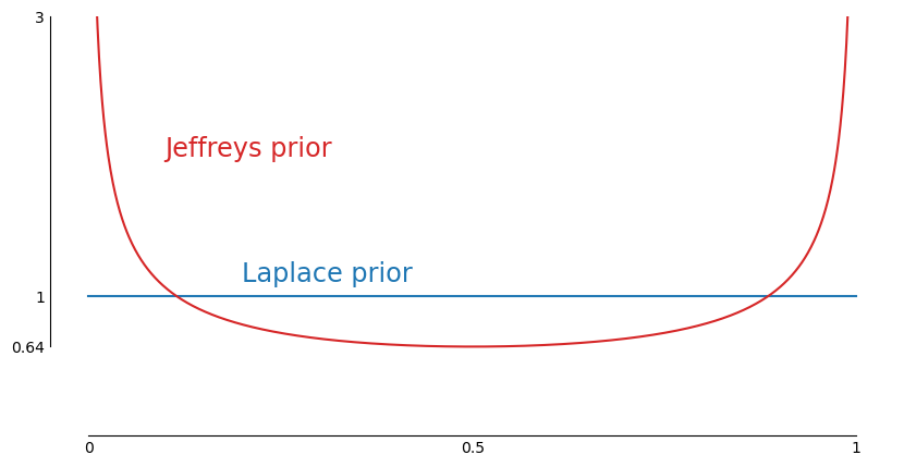
The posterior is then

which we can recognize as the beta distribution with parameters y+1/2 and n-y+1/2.

To test frequentist coverages, we can use an exact algorithm.

function binomial-coverage-test(n, θ_true, α):
  cov ← 0
  for y ← 0 to n do
    t ← integrate_0^θ_true π(θ | y)dθ
    if (1 - α)/2 < t < 1 - (1 - α)/2:
      cov ← cov + binomial_coefficient(n, y) * θ_true^y * (1 - θ_true)^(n-y)
    end if
  end for
  return cov

Here are the coverage results for α=0.95 and various values of p and n using the Bayes-Laplace uniform prior:

and here are the coverage results using Jeffreys prior:

We can see coverage is identical for many table entries. For smaller values of n and p_true, though, the uniform prior gives no coverage while Jeffreys prior provides decent results. [source code for experiment]

Applications from Bayes and Laplace

Let’s now revisit some applications Bayes and Laplace studied. Given that the goal in all of these problems is to assign a belief probability to an interval of the parameter space, I think that we can make a strong argument that Jeffreys prior is a better choice than the uniform prior since it has asymptotically optimal frequentist coverage performance. This also addresses Fisher’s criticism of arbitrariness.

Note: See [14, p. 105–106] for a more through discussion of the uniform prior vs Jeffreys prior for the binomial distribution

In each of these problems, I’ll show both the answer given by Jeffreys prior and the original uniform prior that Bayes and Laplace used. One theme we’ll see is that many of the results are not that different. A lot of fuss is often made over minor differences in how objective priors can be derived. The differences can be important, but often the data dominates and different reasonable choices will lead to nearly the same result.

Example 3: Observing Only 1s

In an appendix Richard Price added to Bayes’ essay, he considers the following problem:

Let us then first suppose, of such an event as that called M in the essay, or an event about the probability of which, antecedently to trials, we know nothing, that it has happened once, and that it is enquired what conclusion we may draw from hence with respct to the probability of it’s happening on a second trial. [4, p. 16]

Specifically, Price asks, “what’s the probability that θ is greater than 1/2?” Using the uniform prior in Bayes’ essay, we derive the posterior distribution

Integrating gives us the answer

Using Jeffreys prior, we derive a beta distribution for the posterior

and the answer

Price then continues with the same problem but supposes we see two 1s, three 1s, etc. The table below shows the result we’d get up to ten 1s. [source code]

Example 4: A Lottery

Price also considers a lottery with an unknown chance of winning:

Let us then imagine a person present at the drawing of a lottery, who knows nothing of its scheme or of the proportion of Blanks to Prizes in it. Let it further be supposed, that he is obliged to infer this from the number of blanks he hears drawn compared with the number of prizes; and that it is enquired what conclusions in these circumstances he may reasonably make. [4, p. 19–20]

He asks this specific question:

Let him first hear ten blanks drawn and one prize, and let it be enquired what chance he will have for being right if he gussses that the proportion of blanks to prizes in the lottery lies somewhere between the proportions of 9 to 1 and 11 to 1. [4, p. 20]

With Bayes prior and θ representing the probability of drawing a blank, we derive the posterior distribution

and the answer

Using Jeffreys prior, we get the posterior

and the answer

Price then considers the same question (what’s the probability that θ lies between 9/10 and 11/12) for different cases where an observer of the lottery sees w prizes and 10w blanks. Below I show posterior probabilities using both Bayes’ uniform prior and Jeffreys prior for various values of w. [source code]

Example 5: Birth Rates

Let’s now turn to a problem that fascinated Laplace and his contemporaries: The relative birth rate of boys-to-girls. Laplace introduces the problem,

The consideration of the [influence of past events on the probability of future events] leads me to speak of births: as this matter is one of the most interesting in which we are able to apply the Calculus of probabilities, I manage so to treat with all care owing to its importance, by determining what is, in this case, the influence of the observed events on those which must take place, and how, by its multiplying, they uncover for us the true ratio of the possibilities of the births of a boy and of a girl. [18, p. 1]

Like Bayes, Laplace approaches the problem using a uniform prior, writing

When we have nothing given a priori on the possibility of an event, it is necessary to assume all the possibilities, from zero to unity, equally probable; thus, observation can alone instruct us on the ratio of the births of boys and of girls, we must, considering the thing only in itself and setting aside the events, to assume the law of possibility of the births of a boy or of a girl constant from zero to unity, and to start from this hypothesis into the different problems that we can propose on this object. [18, p. 26]

Using data collection from Paris between 1745 and 1770, where 251527 boys and 241945 girls had been born, Laplace asks, what is “the probability that the possibility of the birth of a boy is equal or less than 1/2“?

With a uniform prior, B = 251527, G = 241945, and θ representing the probability that a boy is born, we obtain the posterior

and the answer

With Jeffreys prior, we similarly derive the posterior

and the answer

Here’s some simulated data using p_true = B / (B + G) that shows how the answers might evolve as more births are observed.

Discussion

Q1: Where does objective Bayesian analysis belong in statistics?

I think Jeffreys was right and standard statistical procedures should deliver “results of the kind we need”. While Bayes and Laplace might not have been fully justified in their choice of a uniform prior, they were correct in their objective of quantifying results in terms of degree of belief. The approach Jeffreys outlined (and was later evolved with reference priors) gives us a pathway to provide “results of the kind we need” while addressing the arbitrariness of a uniform prior. Jeffreys approach isn’t the only way to get to results as degrees of belief, and a more subjective approach can also be valid if the situation allows, but his approach give us good answers for the common case “of an event concerning the probability of which we absolutely know nothing” and can be used as a drop-in replacement for frequentist methods.

To answer more concretely, I think when you open up a standard introduction-to-statistics textbook and look up a basic procedure such as a hypothesis test of whether the mean of normally distributed data with unknown variance is non-zero, you should see a method built on objective priors and Bayes factor like [19] rather than a method based on P values.

Q2: But aren’t there multiple ways of deriving good priors in the absence of prior knowledge?

I highlighted frequentist coverage matching as a benchmark to gauge whether a prior is a good candidate for objective analysis, but coverage matching isn’t the only valid metric we could use and it may be possible to derive multiple priors with good coverage. Different priors with good frequentist properties, though, will likely be similar, and any results will be determined more by observations than the prior. If we are in a situation where multiple good priors lead to significantly differing results, then that’s an indicator we need to provide subjective input to get a useful answer. Here’s how Berger addresses this issue:

Inventing a new criterion for finding “the optimal objective prior” has proven to be a popular research pastime, and the result is that many competing priors are now available for many situations. This multiplicity can be bewildering to the casual user.

I have found the reference prior approach to be the most successful approach, sometimes complemented by invariance considerations as well as study of frequentist properties of resulting procedures. Through such considerations, a particular prior usually emerges as the clear winner in many scenarios, and can be put forth as the recommended objective prior for the situation. [20]

Q3. Doesn’t that make inverse probability subjective, whereas frequentist methods provide an objective approach to statistics?

It’s a common misconception that frequentist methods are objective. Berger and Berry provides this example to demonstrate [21]: Suppose we watch a research study a coin for bias. We see the researcher flip the coin 17 times. Heads comes up 13 times and tails comes up 4 times. Suppose θ represents the probability of heads and the researcher is doing a standard P-value test with the null hypothesis that the coin is not bias, θ=0.5. What P-value would they get? We can’t answer the question because the researcher would get remarkably different results depending on their experimental intentions.

If the researcher intended to flip the coin 17 times, then the probability of seeing a value less extreme than 13 heads under the null hypothesis is given by summing binomial distribution terms representing the probabilities of getting 5 to 12 heads,

which gives us a P-value of 1–0.951=0.049.

If, however, the researcher intended to continue flipping until they got at least 4 heads and 4 tails, then the probability of seeing a value less extreme than 17 total flips under the null hypothesis is given by summing negative binomial distribution terms representing the probabilities of getting 8 to 16 total flips,

which gives us a P-value of 1–0.979=0.021

The result is dependent on not just the data but also on the hidden intentions of the researcher. As Berger and Berry argue “objectivity is not generally possible in statistics and … standard statistical methods can produce misleading inferences.” [21] [source code for example]

Q4. If subjectivity is unavoidable, why not just use subjective priors?

When subjective input is possible, we should incorporate it. But we should also acknowledge that Bayes’ “event concerning the probability of which we absolutely know nothing” is an important fundamental problem of inference that needs good solutions. As Edwin Jaynes writes

To reject the question, [how do we find the prior representing “complete ignorance”?], as some have done, on the grounds that the state of complete ignorance does not “exist” would be just as absurd as to reject Euclidean geometry on the grounds that a physical point does not exist. In the study of inductive inference, the notion of complete ignorance intrudes itself into the theory just as naturally and inevitably as the concept of zero in arithmetic.

If one rejects the consideration of complete ignorance on the grounds that the notion is vague and ill-defined, the reply is that the notion cannot be evaded in any full theory of inference. So if it is still ill-defined, then a major and immediate objective must be to find a precise definition which will agree with intuitive requirements and be of constructive use in a mathematical theory. [22]

Moreover, systematic approaches such as reference priors can certainly do much better than pseudo-Bayesian techniques such as choosing a uniform prior over a truncated parameter space or a vague proper prior such as a Gaussian over a region of the parameter space that looks interesting. Even when subjective information is available, using reference priors as building blocks is often the best way to incorporate it. For instance, if we know that a parameter is restricted to a certain range but don’t know anything more, we can simply adapt a reference prior by restricting and renormalizing it [14, p. 256].

Note: The term pseudo-Bayesian comes from [20]. See that paper for a more through discussion and comparison with objective Bayesian analysis.

Conclusion

The common and repeated misinterpretation of statistical results such as P values or confidence intervals as belief probabilities shows us that there is a strong natural tendency to want to think about inference in terms of inverse probability. It’s no wonder that the method dominated for 150 years.

Fisher and others were certainly correct to criticize naive use of a uniform prior as arbitrary, but this is largely addressed by reference priors and adopting metrics like frequentist matching coverage that quantify what it means for a prior to represent ignorance. As Berger puts it,

We would argue that noninformative prior Bayesian analysis is the single most powerful method of statistical analysis, in the sense of being the ad hoc method most likely to yield a sensible answer for a given investment of effort. And the answers so obtained have the added feature of being, in some sense, the most “objective” statistical answers obtainable [23, p. 90]

Notes & References

[1]: Problem of the points: Suppose two players A and B each contribute an equal amount of money into a prize pot. A and B then agree to play repeated rounds of a game of chance, with the players having an equal probability of winning any round, until one of the players has won k rounds. The player that first reaches k wins takes the entirety of the prize pot. Now, suppose the game is interrupted with neither player reaching k wins. If A has w_A wins and B has w_B wins, what’s a fair way to split the pot?

[2]: Bernoulli, J. (1713). On the Law of Large Numbers, Part Four of Ars Conjectandi. Translated by Oscar Sheynin.

[3]: De Moivre, A. (1756). The Doctrine of Chances.

[4]: Bayes, T. (1763). An essay towards solving a problem in the doctrine of chances. by the late rev. mr. bayes, f. r. s. communicated by mr. price, in a letter to john canton, a. m. f. r. s. Philosophical Transactions of the Royal Society of London 53, 370–418.

[5]: Stigler, S. (1990). The History of Statistics: The Measurement of Uncer- tainty before 1900. Belknap Press.

[6]: Laplace, P. (1774). Memoir on the probability of the causes of events. Translated by S. M. Stigler.

[7]: De Morgan, A. (1838). An Essay On Probabilities: And On Their Application To Life Contingencies And Insurance Offices.

[8]: Fisher, R. (1930). Inverse probability. Mathematical Proceedings of the Cambridge Philosophical Society 26(4), 528–535.

[9]: Fisher, R. (1922). On the mathematical foundations of theoretical statistics. Philosophical Transactions of the Royal Society of London. Series A, Containing Papers of a Mathematical or Physical Character 222, 309–368.

[10]: Jeffreys, H. (1961). Theory of Probability (3 ed.). Oxford Classic Texts in the Physical Sciences.

[11]: Welch, B. L. and H. W. Peers (1963). On formulae for confidence points based on integrals of weighted likelihoods. Journal of the Royal Statistical Society Series B-methodological 25, 318–329.

[12]: Goodman, S. (1999, June). Toward evidence-based medical statistics. 1: The p value fallacy. Annals of Internal Medicine 130 (12), 995–1004.

[13]: Berger, J. O., J. M. Bernardo, and D. Sun (2009). The formal definition of reference priors. The Annals of Statistics 37 (2), 905–938.

[14]: Berger, J., J. Bernardo, and D. Sun (2024). Objective Bayesian Inference. World Scientific.

[15]: Berger, J. and T. Sellke (1987). Testing a point null hypothesis: The irreconcilability of p values and evidence. Journal of the American Statistical Association 82(397), 112–22.

[16]: Selke, T., M. J. Bayarri, and J. Berger (2001). Calibration of p values for testing precise null hypotheses. The American Statistician 855(1), 62–71.

[17]: Berger, J., J. Bernardo, and D. Sun (2022). Objective bayesian inference and its relationship to frequentism.

[18]: Laplace, P. (1778). Mémoire sur les probabilités. Translated by Richard J. Pulskamp.

[19]: Berger, J. and J. Mortera (1999). Default bayes factors for nonnested hypothesis testing. Journal of the American Statistical Association 94 (446), 542–554.

[20]: Berger, J. (2006). The case for objective Bayesian analysis. Bayesian Analysis 1(3), 385–402.

[21]: Berger, J. O. and D. A. Berry (1988). Statistical analysis and the illusion of objectivity. American Scientist 76(2), 159–165.

[22]: Jaynes, E. T. (1968). Prior probabilities. Ieee Transactions on Systems and Cybernetics (3), 227–241.

[23]: Berger, J. (1985). Statistical Decision Theory and Bayesian Analysis. Springer.

[24]: The portrait of Thomas Bayes is in the public domain; the portrait of Pierre-Simon Laplace is by Johann Ernst Heinsius (1775) and licensed under Creative Commons Attribution-Share Alike 4.0 International; and use of Harold Jeffreys portrait qualifies for fair use.

[25]: Zabell, S. (1989). R. A. Fisher on the History of Inverse Probability. Statistical Science 4(3), 247–256.

---

An Introduction to Objective Bayesian Inference was originally published in Towards Data Science on Medium, where people are continuing the conversation by highlighting and responding to this story.