Tag: tech

  • Robust One-Hot Encoding

    Robust One-Hot Encoding

    Hans Christian Ekne

    Production grade one-hot encoding techniques in Python and R

    Image generated by the author using DALL-E / or Dali?;)

    Have you faced a crash in your machine learning production environments?

    It’s not fun, and especially when it comes to issues that could be avoided. One issue that frequently causes problems is one-hot encoding of data. Drawing from my own experience, I’ve learned that many of these issues can largely be avoided by following a few best practices related to one-hot encoding. In this article I will briefly introduce the topic with a few simple examples and share some best practices to ensure stability of your machine learning models.

    One-hot encoding

    What is one-hot encoding?

    One-hot encoding is the practice of turning a factor variable that is stored in a column into dummy variables stored over multiple columns and represented as 0s and 1s. A simple example illustrates the concept.

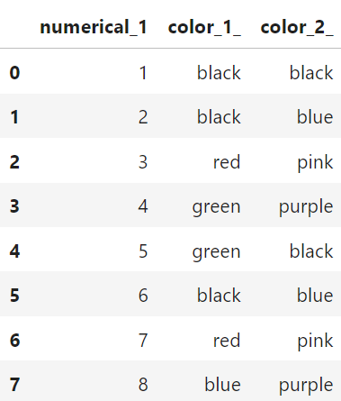
    Consider for example this dataset with some numbers and some columns for colours:

    import pandas as pd

    # Creating the training_data DataFrame in Python
    training_data = pd.DataFrame({
    'numerical_1': [1, 2, 3, 4, 5, 6, 7, 8],
    'color_1_': ['black', 'black', 'red', 'green',
    'green', 'black', 'red', 'blue'],
    'color_2_': ['black', 'blue', 'pink', 'purple',
    'black', 'blue', 'pink', 'purple']
    })

    Or more visually:

    Training data with 3 columns / image by author

    The column color_1_could also be represented like in the table below:

    encoded variables of color_1
    One-hot encoded representation of “color_1_” / image by author

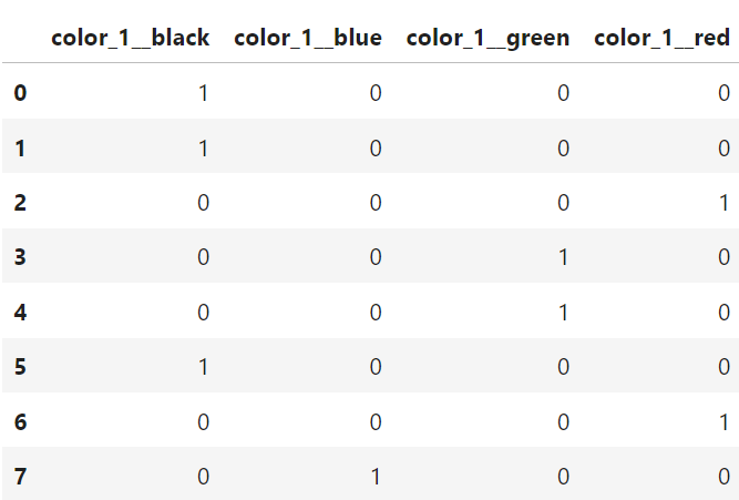
    Changing color_1_ from a one-column compact representation of a categorical variable into a multi-column binary representation is what we call one-hot encoding.

    Why do we use it?

    There are multiple reasons to use one-hot encoding. They could be related to avoiding implicit ordering, improving model performance, or just making the data compatible with various algorithms.

    For example, when you encode a categorical variable like colour, into a numerical structure, (e.g. 1 for black, 2 for green, 3 for red) without converting it to dummy variables, a model could mistakenly misinterpret the data to imply an order ( black < green < red) when no such order exists.

    Also, when training neural nets, it is best practice to normalize the data before sending it into the neural net, and with categorical variables, one-hot encoding can be a good method. Other linear models, like logistic and linear regression assume linear relationships and numerical inputs so for this class of models, one-hot encoding can be a good idea as well.

    In addition, the process of doing one-hot encoding forces us to ensure we don’t feed unseen factor levels into our machine learning models.

    Ultimately, one-hot encoding makes it easier for the machine learning models to interpret the data and thus make better predictions.

    The main reasons why one-hot encoding fails

    The way we build traditional machine learning models is to first train the models on a “training dataset” — typically a dataset of historic values — and then later we generate predictions on a new dataset, the “inference dataset.” If the columns of the training dataset and the inference dataset don’t match, your machine learning algorithm will usually fail. This is primarily due to either missing or new factor levels in the inference dataset.

    The first problem: Missing factors

    For the following examples, assume that you used the dataset above to train your machine learning model. You one-hot encoded the dataset into dummy variables, and your fully transformed training data looks like below:

    Transformed training dataset with pd.get_dummies / image by author

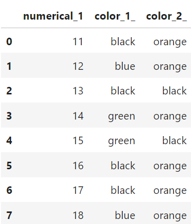
    Now, let’s introduce the inference dataset, this is what you would use for making predictions. Let’s say it is given like below:

    # Creating the inference_data DataFrame in Python
    inference_data = pd.DataFrame({
    'numerical_1': [11, 12, 13, 14, 15, 16, 17, 18],
    'color_1_': ['black', 'blue', 'black', 'green',
    'green', 'black', 'black', 'blue'],
    'color_2_': ['orange', 'orange', 'black', 'orange',
    'black', 'orange', 'orange', 'orange']
    })
    Inference data with 3 columns / image by author

    Using a naive one-hot encoding strategy like we used above (pd.get_dummies)

    # Converting categorical columns in inference_data to 
    # Dummy variables with integers
    inference_data_dummies = pd.get_dummies(inference_data,
    columns=['color_1_', 'color_2_']).astype(int)

    This would transform your inference dataset in the same way, and you obtain the dataset below:

    Transformed inference dataset with pd.get_dummies / image by author

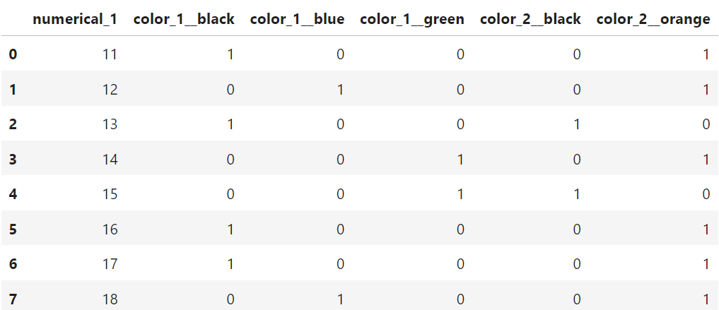
    Do you notice the problems? The first problem is that the inference dataset is missing the columns:

    missing_colmns =['color_1__red', 'color_2__pink', 
    'color_2__blue', 'color_2__purple']

    If you ran this in a model trained with the “training dataset” it would usually crash.

    The second problem: New factors

    The other problem that can occur with one-hot encoding is if your inference dataset includes new and unseen factors. Consider again the same datasets as above. If you examine closely, you see that the inference dataset now has a new column: color_2__orange.

    This is the opposite problem as previously, and our inference dataset contains new columns which our training dataset didn’t have. This is actually a common occurrence and can happen if one of your factor variables had changes. For example, if the colours above represent colours of a car, and a car producer suddenly started making orange cars, then this data might not be available in the training data, but could nonetheless show up in the inference data. In this case you need a robust way of dealing with the issue.

    One could argue, well why don’t you list all the columns in the transformed training dataset as columns that would be needed for your inference dataset? The problem here is that you often don’t know what factor levels are in the training data upfront.

    For example, new levels could be introduced regularly, which could make it difficult to maintain. On top of that comes the process of then matching your inference dataset with the training data, so you would need to check all actual transformed column names that went into the training algorithm, and then match them with the transformed inference dataset. If any columns were missing you would need to insert new columns with 0 values and if you had extra columns, like the color_2__orange columns above, those would need to be deleted. This is a rather cumbersome way of solving the issue, and thankfully there are better options available.

    The solution

    The solution to this problem is rather straightforward, however many of the packages and libraries that attempt to streamline the process of creating prediction models fail to implement it well. The key lies in having a function or class that is first fitted on the training data, and then use that same instance of the function or class to transform both the training dataset and the inference dataset. Below we explore how this is done using both Python and R.

    In Python

    Python is arguably one the best programming language to use for machine learning, largely due to its extensive network of developers and mature package libraries, and its ease of use, which promotes rapid development.

    Regarding the issues related to one-hot encoding we described above, they can be mitigated by using the widely available and tested scikit-learn library, and more specifically the sklearn.preprocessing.OneHotEncoder class. So, let’s see how we can use that on our training and inference datasets to create a robust one-hot encoding.

    from sklearn.preprocessing import OneHotEncoder

    # Initialize the encoder
    enc = OneHotEncoder(handle_unknown='ignore')

    # Define columns to transform
    trans_columns = ['color_1_', 'color_2_']

    # Fit and transform the data
    enc_data = enc.fit_transform(training_data[trans_columns])

    # Get feature names
    feature_names = enc.get_feature_names_out(trans_columns)

    # Convert to DataFrame
    enc_df = pd.DataFrame(enc_data.toarray(),
    columns=feature_names)

    # Concatenate with the numerical data
    final_df = pd.concat([training_data[['numerical_1']],
    enc_df], axis=1)

    This produces a final DataFrameof transformed values as shown below:

    Transformed training dataset with sklearn / image by author

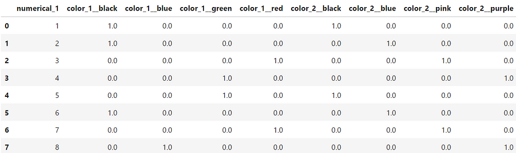
    If we break down the code above, we see that the first step is to initialize the an instance of the encoder class. We use the option handle_unknown=’ignore’ so that we avoid issues with unknow values for the columns when we use the encoder to transform on our inference dataset.

    After that, we combine a fit and transform action into one step with the fit_transform method. And finally, we create a new data frame from the encoded data and concatenate it with the rest of the original dataset.

    Now the task remains to use the encoder to transform our inference dataset.

    # Transform inference data
    inference_encoded = enc.transform(inference_data[trans_columns])

    inference_feature_names = enc.get_feature_names_out(trans_columns)

    inference_encoded_df = pd.DataFrame(inference_encoded.toarray(),
    columns=inference_feature_names)

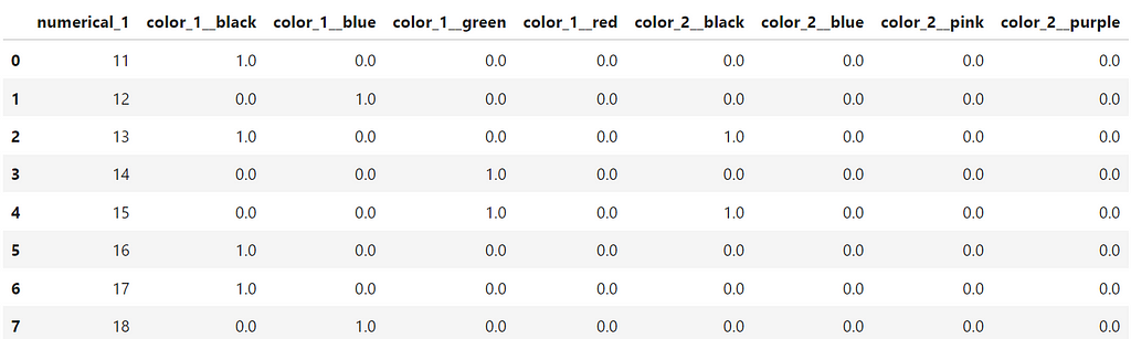
    final_inference_df = pd.concat([inference_data[['numerical_1']],
    inference_encoded_df], axis=1)

    Unlike earlier, when we used the naive pandas.get_dummies ,we now see that our new final_inference_df dataset has the same columns as our training dataset.

    Transformed Inference dataset with the correct columns / image by author

    In addition to what we showed in the code above, the OneHotEncoder class from sklearn.preprocessing has a lot of other functionality that can be useful as well.

    For example, it allows you set the min_frequency and max_categories options. As its name implies the min_frequency options allow you to specify the minimum frequency below which a category will be considered infrequent and then grouped together with other infrequent categories, or the max_categories option which limits the total number of categories. The latter can be especially useful if you don’t want to create too many columns in your training dataset.

    For a full overview of the functionality, visit the documentation pages here:

    sklearn.preprocessing.OneHotEncoder

    In R

    Several of my clients use R for running machine learning models in production — and it has a lot of great features. Before polars came out for Python, R’s data.table package was superior to what pandas could offer in terms of speed and efficiency. However, R doesn’t have access to the same type of production level packages as scikit-learn for python. (There are a few libraries, but they are not as mature as scikit-learn.) In addition, while some packages might have the required functionality, they require loads of other packages to run and can introduce dependency conflicts into your code. Consider running the line below in a docker container build with the r-base image:

    RUN R -e "install.packages('recipes', dependencies=TRUE, repos='https://cran.rstudio.com/')"

    It takes forever to install and takes up a lot of space on your container image. Our solution in this case — instead of using functions from a pre-built package like recipes — is to introduce our own simple function implemented using the data.table package:

    library(data.table)

    OneHotEncoder <- function() {
    # Local variables
    categories <- list()

    # Method to fit data and extract categories
    fit <- function(dt, columns) {
    for (column in columns) {
    categories[[column]] <<- unique(dt[[column]])
    }
    }

    # Method to turn columns into factors and
    factorize <- function(dt) {
    for (column_name in names(categories)) {
    set(dt, j = column_name,
    value = factor(dt[[column_name]],
    levels = categories[[column_name]]))
    }
    return(dt)
    }

    # Method to transform columns in categories list to
    # dummy variables
    transform <- function(dt) {
    dt = factorize(dt)
    # add row number for joins later
    dt[, rn := .I]
    for (col in names(categories)) {
    print(col)
    # Construct the formula dynamically
    formula_str <- paste("~", col, "- 1")
    formula_obj <- as.formula(formula_str)
    # Create a model model.matrix object
    mm = model.matrix(formula_obj, dt)
    mm_dt <- as.data.table(mm, keep.rownames = "rn")
    mm_dt[, rn := as.integer(rn)]

    # Perform a merge based on these row numbers
    dt <- merge(dt, mm_dt, by = "rn", all = TRUE)

    # remove the original column
    dt[, (col) := NULL]

    # set any new NAs to 0
    for (ncol in names(mm_dt)) {
    set(dt, which(is.na(dt[[ncol]])), ncol, 0)
    }
    }
    dt[, rn := NULL]
    return(dt)
    }

    # Method to get categories
    get_categories <- function() {
    return(categories)
    }

    # Return a list of methods
    list(
    get_categories = get_categories,
    fit = fit,
    transform = transform
    )
    }

    Let’s go through this function and see how it works on our training and inference datasets. (R is slightly different from Python and instead of using a class, we use a parent function instead, which works in a similar way.)

    First, we need to create an instance of the function:

     encoder = OneHotEncoder()

    Then, just like with the OneHotEncoder class from sklearn.preprocessing, we also have a fit function inside our OneHotEncoder. We use the fit function on the training data, supplying both the training dataset and the columns we want to one-hot encode.

    # Columns to one-hot encode
    fit_columns = c("color_1_", "color_2")
    # Use the fit method
    encoder$fit(dt=training_data, columns=fit_columns)

    The fit function simply loops through all the columns we want to use to for training and finds all the unique values each of the columns contain. This list of columns and their potential values is then used in the transform function. We now have a instance of a fitted one-hot encoder function and we can save it for later use using a R .RDS file.

    saveRDS(encoder, "~/my_encoder.RDS")

    To generate the one-hot encoded dataset we need for training, we run the transform function on the training data:

    transformed_training_data = encoder$transform(training_data)

    The transform function is a little bit more complicated than the fit function, and the first thing it does is to convert the supplied columns into factors — using the original unique values of the columns as factor levels. Then, we loop through each of the predictor columns and create model.matrix objects of the data. These are then added back to the original dataset and the original factor column is removed. We also make sure to set any of the missing values to 0.

    We now get the exact same dataset as before:

    Transformed training dataset using R algorithm / image by author

    And finally, when we need to one-hot encode our inference dataset, we then run the same instance of the encoder function on that dataset:

    transformed_inference_data = encoder$transform(inference_data)

    This process ensures we have the same columns in our transformed_inference_data as we do in our transformed_training_data.

    Further considerations

    Before we conclude there are a few extra considerations to mention. As with many other things in machine learning there isn’t always an easy answer as to when and how to use a specific technique. Even though it clearly mitigates some issues, new problems can also arise when doing one-hot encoding. Most commonly, these are related to how to deal with high cardinality categorical variables and how to deal with memory issues because of increasing the table size.

    In addition, there are alternative coding techniques such as label encoding, embeddings, or target encodings which sometimes could be preferable to one-hot encoding.

    Each of these topics is rich enough to warrant a dedicated article, so we will leave those for the interested reader to explore further.

    Conclusion

    We have shown how naive use of one-hot encoding techniques can lead to mistakes and problems with inference data, and we have also seen how to mitigate and resolve those issues using both Python and R. If left unresolved, poor management of one-hot encoding can potentially lead to crashes and problems with your inference, so it is strongly recommended to use more robust techniques—like either sklearn’s OneHotEncoder or the R function we developed.

    Thanks for reading!

    All the code presented and used in the article can be found in the following Github repo: https://github.com/hcekne/robust_one_hot_encoding

    If you enjoyed reading this article and would like to access more content from me please feel free to connect with me on LinkedIn at https://www.linkedin.com/in/hans-christian-ekne-1760a259/ or visit my webpage at https://www.ekneconsulting.com/ to explore some of the services I offer. Don’t hesitate to reach out via email at [email protected]


    Robust One-Hot Encoding was originally published in Towards Data Science on Medium, where people are continuing the conversation by highlighting and responding to this story.

    Originally appeared here:
    Robust One-Hot Encoding

    Go Here to Read this Fast! Robust One-Hot Encoding

  • Temperature Scaling and Beam Search Text Generation in LLMs, for the ML-Adjacent

    Temperature Scaling and Beam Search Text Generation in LLMs, for the ML-Adjacent

    Mike Cvet

    What “temperature” is, how it works, its relationship to the beam search heuristic, and how LLM output generation can still go haywire

    Photo by Paul Green on Unsplash; all other images by author unless otherwise noted

    If you’ve spent any time with APIs for LLMs like those from OpenAI or Anthropic, you’ll have seen the temperature setting available in the API. How is this parameter used, and how does it work?

    From the Anthropic chat API documentation:

    temperature (number)

    Amount of randomness injected into the response.

    Defaults to 1.0. Ranges from 0.0 to 1.0. Use temperature closer to 0.0 for
    analytical / multiple choice, and closer to 1.0 for creative and
    generative tasks.

    Note that even with temperature of 0.0, the results will not be
    fully deterministic.

    Temperature (as is generally implemented) doesn’t really inject randomness into the response. In this post, I’ll walk through what this setting does, and how it’s used in beam search, the most common text generation technique for LLMs, as well as demonstrate some output-generation examples (failures and successes) using a reference implementation in Github.

    What you’re getting yourself into:

    Revisiting LLM Inference and Token Prediction

    If you’re here, you probably have some understanding of how LLMs work.

    At a high level, LLM text generation involves predicting the next token in a sequence, which depends on the cumulative probability of the preceding tokens. This process utilizes internal probability distributions that are shaped by:

    • The model’s internal, learned weights, refined through extensive training on vast datasets
    • The entire input context (the query and any other augmenting data or documents)
    • The set of tokens generated thus far

    Transformer-based generative models build representations of their input contexts through Self-Attention, allowing them to dynamically assess and prioritize different parts of the input based on their relevance to the current prediction point. During sequence decoding, these models evaluate how each part of the input influences the emerging sequence, ensuring that each new token reflects an integration of both the input and the evolving output (largely through Cross-Attention).

    The Stanford CS224N course materials are a great resource for these concepts.

    The key point I want to make here is that when the model decides on the probabilistically best token, it’s generally evaluating the entire input context, as well as the entire generated sequence in-progress. However, the most intuitive process for using these predictions to iteratively build text sequences is simplistic: a greedy algorithm, where the output text is built based on the most-likely token at every step.

    Below I’ll discuss how it works, where it fails, and some techniques used to adapt to those failures.

    Greedy Search

    The most natural way to use a model to build an output sequence is to gradually predict the next-best token, append it to a generated sequence, and continue until the end of generation. This is called greedy search, and is the most simple and efficient way to generate text from an LLM (or other model). In its most basic form, it looks something like this:

    sequence = ["<start>"]
    while sequence[-1] != "<end>":
    # Given the input context, and seq so far, append most likely next token
    sequence += model(input, sequence)
    return "".join(sequence)

    Undergrad Computer Science algorithms classes have a section on graph traversal algorithms. If you model the universe of potential LLM output sequences as a graph of tokens, then the problem of finding the optimal output sequence, given input context, closely resembles the problem of traversing a weighted graph. In this case, the edge “weights” are probabilities generated from attention scores, and the goal of the traversal is to minimize the overall cost (maximize the overall probability) from beginning to end.

    Greedy best-first search traverses through the conceptual graph tokens by making the seemingly best possible decision at every step in a forwards-only direction

    Out of all possible text generation methods, this is the most computationally efficient — the number of inferences is 1:1 with the number of output tokens. However, there are some problems.

    At every step of token generation, the algorithm selects the highest-probability token given the output sequence so far, and appends it to that sequence. This is the simplicity and flaw of this approach, along with all other greedy algorithms — it gets trapped in local minima. Meaning, what appears to be the next-best token right now may not, in fact, be the next-best token for the generated output overall.

    "We can treat it as a matter of" 
    [course (p=0.9) | principle (p=0.5)] | cause (p=0.2)]"

    Given some input context and the generated string so far, We can treat it as a matter of course seems like a logical and probable sequence to generate.

    But what if the contextually-accurate sentence is We can treat it as a matter of cause and effect? Greedy search has no way to backtrack and rewrite the sequence token course with cause and effect. What seemed like the best token at the time actually trapped output generation into a suboptimal sequence.

    The need to account for lower-probability tokens at each step, in the hope that better output sequences are generated later, is where beam search is useful.

    Beam Search

    Returning to the graph-search analogy, in order to generate the optimal text for any given query and context, we’d have to fully explore the universe of potential token sequences. The solution resembles the A* search algorithm (more closely than Dijkstra’s algorithm, since we don’t necessarily want shortest path, but lowest-cost/highest-likelihood).

    A* search illustration by Wgullyn from https://en.wikipedia.org/wiki/A*_search_algorithm

    Since we’re working with natural language, the complexity involved is far too high to exhaust the search space for every query in most contexts. The solution is to trim that search space down to a reasonable number of candidate paths through the candidate token graph; maybe just 4, 8, or 12.

    Beam search is the heuristic generally used to approximate that ideal A*-like outcome. This technique maintains k candidate sequences which are incrementally built up with the respective top-k most likely tokens. Each of these tokens contributes to an overall sequence score, and after each step, the total set of candidate sequences are pruned down to the best-scoring top k.

    Beam search, similarly to A* search, maintains multiple paths from start to end, evaluating the overall score of a limited number of candidate sequences under evaluation. The number is referred to as the “beam width”.

    The “beam” in beam search borrows the analogy of a flashlight, whose beam can be widened or narrowed. Taking the example of generating the quick brown fox jumps over the lazy dog with a beam width of 2, the process looks something like this:

    At this step, two candidate sequences are being maintained: “the” and “a”. Each of these two sequences need to evaluate the top-two most likely tokens to follow.

    After the next step, “the speedy” has been eliminated, and “the quick” has been selected as the first candidate sequence. For the second, “a lazy” has been eliminated, and “a quick” has been selected, as it has a higher cumulative probability. Note that if both candidates above the line have a higher likelihood that both candidates below the line, then they will represent the two candidate sequences after the subsequent step.

    This process continues until either a maximum token length limit has been reached, or all candidate sequences have appended an end-of-sequence token, meaning we’ve concluded generating text for that sequence.

    Increasing the beam width increases the search space, increasing the likelihood of a better output, but at a corresponding increase space and computational cost. Also note that a beam search with beam_width=1 is effectively identical to greedy search.

    Temperature

    Now, what does temperature have to do with all of this? As I mentioned above, this parameter doesn’t really inject randomness into the generated text sequence, but it does modify the predictability of the output sequences. Borrowing from information theory: temperature can increase or decrease the entropy associated with a token prediction.

    The softmax activation function is typically used to convert the raw outputs (ie, logits) of a model’s (including LLMs) prediction into a probability distribution (I walked through this a little here). This function is defined as follows, given a vector Z with n elements:

    Theta is generally used to refer to the softmax function

    This function emits a vector (or tensor) of probabilities, which sum to 1.0 and can be used to clearly assess the model’s confidence in a class prediction in a human-interpretable way.

    A “temperature” scaling parameter T can be introduced which scales the logit values prior to the application of softmax.

    The application of the temperature scaling parameter T to the inputs to the softmax function

    The application of T > 1.0 has the effect of scaling down logit values and produces the effect of the muting the largest differences between the probabilities of the various classes (it increases entropy within the model’s predictions)

    Using a temperature of T < 1.0 has the opposite effect; it magnifies the differences, meaning the most confident predictions will stand out even more compared to alternatives. This reduces the entropy within the model’s predictions.

    In code, it looks like this:

    scaled_logits = logits_tensor / temperature
    probs = torch.softmax(scaled_logits, dim=-1)

    Take a look at the effect over 8 possible classes, given some hand-written logit values:

    Generated via the script in my linked repository

    The above graph was plotted using the following values:

    ts = [0.5, 1.0, 2.0, 4.0, 8.0]
    logits = torch.tensor([3.123, 5.0, 3.234, 2.642, 2.466, 3.3532, 3.8, 2.911])
    probs = [torch.softmax(logits / t, dim=-1) for t in ts]

    The bars represent the logit values (outputs from model prediction), and the lines represent the probability distribution over those classes, with probabilities defined on the right-side label. The thick red line represents the expected distribution, with temperature T=1.0, while the other lines demonstrate the change in relative likelihood with a temperature range from 0.5 to 8.0.

    You can clearly see how T=0.5 emphasizes the likelihood of the largest-magnitude logit index, while T=8.0 reduces the difference in probabilities between classes to almost nothing.

    >>> [print(f' t={t}n l={(logits/t)}n p={p}n') for p,t in zip(probs, ts)]
    t=0.5
    l=tensor([6.2460, 10.000, 6.4680, 5.2840, 4.9320, 6.7064, 7.6000, 5.8220])
    p=tensor([0.0193, 0.8257, 0.0241, 0.0074, 0.0052, 0.0307, 0.0749, 0.0127])

    t=1.0
    l=tensor([3.1230, 5.0000, 3.2340, 2.6420, 2.4660, 3.3532, 3.8000, 2.9110])
    p=tensor([0.0723, 0.4727, 0.0808, 0.0447, 0.0375, 0.0911, 0.1424, 0.0585])

    t=2.0
    l=tensor([1.5615, 2.5000, 1.6170, 1.3210, 1.2330, 1.6766, 1.9000, 1.4555])
    p=tensor([0.1048, 0.2678, 0.1108, 0.0824, 0.0754, 0.1176, 0.1470, 0.0942])

    t=4.0
    l=tensor([0.7807, 1.2500, 0.8085, 0.6605, 0.6165, 0.8383, 0.9500, 0.7278])
    p=tensor([0.1169, 0.1869, 0.1202, 0.1037, 0.0992, 0.1238, 0.1385, 0.1109])

    t=8.0
    l=tensor([0.3904, 0.6250, 0.4042, 0.3302, 0.3083, 0.4191, 0.4750, 0.3639])
    p=tensor([0.1215, 0.1536, 0.1232, 0.1144, 0.1119, 0.1250, 0.1322, 0.1183])

    Now, this doesn’t necessarily change the relative likelihood between any two classes (numerical stability issues aside), so how does this have any practical effect in sequence generation?

    The answer lies back in the mechanics of beam search. A temperature value greater than 1.0 makes it less likely a high-scoring individual token will outweigh a series of slightly-less-likely tokens, which in conjunction result in a better-scoring output.

    >>> sum([0.9, 0.3, 0.3, 0.3]) # raw probabilities
    1.8 # dominated by first token
    >>> sum([0.8, 0.4, 0.4, 0.4]) # temperature-scaled probabilities
    2.0 # more likely overall outcome

    Implementation Details

    Beam search implementations typically work with log-probabilities of the softmax probabilities, which is common in the ML domain among many others. The reasons include:

    • The probabilities in use are often vanishingly small; using log probs improves numerical stability
    • We can compute a cumulative probability of outcomes via the addition of logprobs versus the multiplication of raw probabilities, which is slightly computationally faster as well as more numerically stable. Recall that p(x) * p(y) == log(p(x)) + log(p(y))
    • Optimizers, such as gradient descent, are simpler when working with log probs, which makes derivative calculations more simple and loss functions like cross-entropy loss already involve logarithmic calculations

    This also means that the values of the log probs we’re using as scores are negative real numbers. Since softmax produces a probability distribution which sums to 1.0, the logarithm of any class probability is thus ≤ 1.0 which results in a negative value. This is slightly annoying, however it is consistent with the property that higher-valued scores are better, while greatly negative scores reflect extremely unlikely outcomes:

    >>> math.log(3)
    1.0986122886681098
    >>> math.log(0.99)
    -0.01005033585350145
    >>> math.log(0.98)
    -0.020202707317519466
    >>> math.log(0.0001)
    -9.210340371976182
    >>> math.log(0.000000000000000001)
    -41.44653167389282

    Here’s most of the example code, highly annotated, also available on Github. Definitions for GeneratedSequence and ScoredToken can be found here; these are mostly simple wrappers for tokens and scores.

    # The initial candidate sequence is simply the start token ID with 
    # a sequence score of 0
    candidate_sequences = [
    GeneratedSequence(tokenizer, start_token_id, end_token_id, 0.0)
    ]

    for i in tqdm.tqdm(range(max_length)):
    # Temporary list to store candidates for the next generation step
    next_step_candidates = []

    # Iterate through all candidate sequences; for each, generate the next
    # most likely tokens and add them to the next-step sequnce of candidates
    for candidate in candidate_sequences:

    # skip candidate sequences which have included the end-of-sequence token
    if not candidate.has_ended():

    # Build a tensor out of the candidate IDs; add a single batch dimension
    gen_seq = torch.tensor(candidate.ids(), device=device).unsqueeze(0)

    # Predict next token
    output = model(input_ids=src_input_ids, decoder_input_ids=gen_seq)

    # Extract logits from output
    logits = output.logits[:, -1, :]

    # Scale logits using temperature value
    scaled_logits = logits / temperature

    # Construct probability distribution against scaled
    # logits through softmax activation function
    probs = torch.softmax(scaled_logits, dim=-1)

    # Select top k (beam_width) probabilities and IDs from the distribution
    top_probs, top_ids = probs.topk(beam_width)

    # For each of the top-k generated tokens, append to this
    # candidate sequence, update its score, and append to the list of next
    # step candidates
    for i in range(beam_width):
    # the new token ID
    next_token_id = top_ids[:, i].item()

    # log-prob of the above token
    next_score = torch.log(top_probs[:, i]).item()

    new_seq = deepcopy(candidate)

    # Adds the new token to the end of this sequence, and updates its
    # raw and normalized scores. Scores are normalized by sequence token
    # length, to avoid penalizing longer sequences
    new_seq.append(ScoredToken(next_token_id, next_score))

    # Append the updated sequence to the next candidate sequence set
    next_step_candidates.append(new_seq)
    else:
    # Append the canddiate sequence as-is to the next-step candidates
    # if it already contains an end-of-sequence token
    next_step_candidates.append(candidate)

    # Sort the next-step candidates by their score, select the top-k
    # (beam_width) scoring sequences and make them the new
    # candidate_sequences list
    next_step_candidates.sort()
    candidate_sequences = list(reversed(next_step_candidates))[:beam_width]

    # Break if all sequences in the heap end with the eos_token_id
    if all(seq.has_ended() for seq in candidate_sequences):
    break

    return candidate_sequences

    In the next section, you can find some results of running this code on a few different datasets with different parameters.

    Greedy Search and Beam Search Generation Examples

    As I mentioned, I’ve published some example code to Github, which uses the t5-small transformer model from Hugging Face and its corresponding T5Tokenizer. The examples below were run through the T5 model against the quick brown fox etc Wikipedia page, sanitized through an extractor script.

    Greedy Search

    Running –greedy mode:

    $ python3 src/main.py --greedy --input ./wiki-fox.txt --prompt "summarize the following document"

    greedy search generation results:
    [
    the phrase is used in the annual Zaner-Bloser National Handwriting Competition.
    it is used for typing typewriters and keyboards, typing fonts. the phrase
    is used in the earliest known use of the phrase.
    ]

    This output summarizes part of the article well, but overall is not great. It’s missing initial context, repeats itself, and doesn’t state what the phrase actually is.

    Beam Search

    Let’s try again, this time using beam search for output generation, using an initial beam width of 4 and the default temperature of 1.0

    $ python3 src/main.py --beam 4 --input ./wiki-fox.txt --prompt "summarize the following document"

    [lots of omitted output]

    beam search (k=4, t=1.0) generation results:
    [
    "the quick brown fox jumps over the lazy dog" is an English-language pangram.
    the phrase is commonly used for touch-typing practice, typing typewriters and
    keyboards. it is used in the annual Zaner-Bloser National
    Handwriting Competition.
    ]

    This output is far superior to the greedy output above, and the most remarkable thing is that we’re using the same model, prompt and input context to generate it.

    There are still a couple mistakes in it; for example “typing typewriters”, and perhaps “keyboards” is ambiguous.

    The beam search code I shared will emit its decision-making progress as it progresses through the text generation (full output here). For example, the first two steps:

    beginning beam search | k = 4 bos = 0 eos = 1 temp = 1.0 beam_width = 4
    0.0: [], next token probabilities:
    p: 0.30537632: ▁the
    p: 0.21197866: ▁"
    p: 0.13339639: ▁phrase
    p: 0.13240208: ▁


    next step candidates:
    -1.18621039: [the]
    -1.55126965: ["]
    -2.01443028: [phrase]
    -2.02191186: []


    -1.1862103939056396: [the], next token probabilities:
    p: 0.61397356: ▁phrase
    p: 0.08461960: ▁
    p: 0.06939770: ▁"
    p: 0.04978605: ▁term


    -1.5512696504592896: ["], next token probabilities:
    p: 0.71881396: the
    p: 0.08922042: qui
    p: 0.05990228: The
    p: 0.03147057: a


    -2.014430284500122: [phrase], next token probabilities:
    p: 0.27810165: ▁used
    p: 0.26313403: ▁is
    p: 0.10535818: ▁was
    p: 0.03361856: ▁


    -2.021911859512329: [], next token probabilities:
    p: 0.72647911: earliest
    p: 0.19509122: a
    p: 0.02678721: '
    p: 0.00308457: s


    next step candidates:
    -1.67401379: [the phrase]
    -1.88142237: ["the]
    -2.34145740: [earliest]
    -3.29419887: [phrase used]
    -3.34952199: [phrase is]
    -3.65579963: [the]
    -3.65619993: [a]

    Now if we look at the set of candidates in the last step:

    next step candidates:
    -15.39409454: ["the quick brown fox jumps over the lazy dog" is an English-language pangram. the phrase is commonly used for touch-typing practice, typing typewriters and keyboards. it is used in the annual Zaner-Bloser National Handwriting Competition.]
    -16.06867695: ["the quick brown fox jumps over the lazy dog" is an English-language pangram. the phrase is commonly used for touch-typing practice, testing typewriters and keyboards. it is used in the annual Zaner-Bloser National Handwriting Competition.]
    -16.10376084: ["the quick brown fox jumps over the lazy dog" is an English-language pangram. the phrase is commonly used for touch-typing practice, typing typewriters and keyboards. it is used in the annual Zaner-Bloser national handwriting competition.]

    You can see that the top-scoring sentence containing typing typewriters outscored the sentence containing testing typewriters by -15.39 to -16.06, which, if we raise to Euler’s constant to convert back into cumulative probabilities, is a probabilistic difference of just 0.00001011316%. There must be a way to overcome this tiny difference!

    Beam Search with Temperature

    Let’s see if this summarization could be improved by applying a temperature value to smooth over some of the log probability scores. Again, everything else, the model, and the input context, will otherwise be identical to the examples above.

    $ python3 src/main.py --beam 4 --temperature 4.0 --input ./wiki-fox.txt --prompt "summarize the following document"

    [lots of omitted output]

    beam search (k=4, t=4.0) generation results:
    [
    "the quick brown fox jumps over the lazy dog" is an English-language pangram.
    it is commonly used for touch-typing practice, testing typewriters and
    computer keyboards. earliest known use of the phrase started with "A"
    ]

    This output correctly emitted “testing typewriters” rather than “typing typewriters” and specified “computer keyboards”. It also, interestingly, chose the historical fact that this phrase originally started with “a quick brown fox” over the Zaner-Bloser competition fact above. The full output is also available here.

    Whether or not this output is better is a subjective matter of opinion. It’s different in a few nuanced ways, and the usage and setting of temperature values will vary by application. I think its better, and again, its interesting because no model weights, model architecture, or prompt was changed to obtain this output.

    Buffalo buffalo Buffalo buffalo buffalo buffalo Buffalo buffalo and Scoring Penalties

    Let’s see if the beam search, with temperature settings used above, works properly for my favorite English-language linguistic construct: Buffalo buffalo Buffalo buffalo buffalo buffalo Buffalo buffalo.

    $ python3 src/main.py --beam 4 --temperature 4.0 --input ./wiki-buffalo.txt --prompt "summarize the linguistic construct in the following text"

    [lots of omitted outputs]

    beam search (k=4, t=4.0) generation results:
    [
    "Buffalo buffalo buffalo buffalo buffalo buffalo buffalo buffalo buffalo
    buffalo buffalo buffalo buffalo buffalo buffalo buffalo buffalo buffalo
    buffalo buffalo buffalo buffalo buffalo buffalo buffalo buffalo buffalo
    buffalo buffalo buffalo buffalo buffalo buffalo buffalo buffalo buffalo
    buffalo buffalo buffalo buffalo buffalo buffalo buffalo buffalo buffalo
    buffalo buffalo buffalo buffalo buffalo buffalo buffalo buffalo buffalo
    buffalo buffalo buffalo buffalo buffalo buffalo
    ]

    Utter disaster, though a predictable one. Given the complexity of this input document, we need additional techniques to handle contexts like this. Interestingly, the final iteration candidates didn’t include a single rational sequence:

    next step candidates:
    -361.66266489: ["Buffalo buffalo buffalo buffalo buffalo buffalo buffalo buffalo buffalo buffalo buffalo buffalo buffalo buffalo buffalo buffalo buffalo buffalo buffalo buffalo buffalo buffalo buffalo buffalo buffalo buffalo buffalo buffalo buffalo buffalo buffalo buffalo buffalo buffalo buffalo buffalo buffalo buffalo buffalo buffalo buffalo buffalo buffalo buffalo buffalo buffalo buffalo buffalo buffalo buffalo buffalo buffalo buffalo buffalo buffalo buffalo buffalo buffalo buffalo buffalo]
    -362.13168168: ["buffalo buffalo buffalo buffalo buffalo buffalo buffalo buffalo buffalo buffalo buffalo buffalo buffalo buffalo buffalo buffalo buffalo buffalo buffalo buffalo buffalo buffalo buffalo buffalo buffalo buffalo buffalo buffalo buffalo buffalo buffalo buffalo buffalo buffalo buffalo buffalo buffalo buffalo buffalo buffalo buffalo buffalo buffalo buffalo buffalo buffalo buffalo buffalo buffalo buffalo buffalo buffalo buffalo buffalo buffalo buffalo buffalo buffalo buffalo buffalo]
    -362.22955942: ["Buffalo buffalo buffalo buffalo buffalo buffalo buffalo buffalo buffalo buffalo buffalo buffalo buffalo buffalo buffalo buffalo buffalo buffalo buffalo buffalo buffalo buffalo buffalo buffalo buffalo buffalo buffalo buffalo buffalo buffalo buffalo buffalo buffalo buffalo buffalo buffalo buffalo buffalo buffalo buffalo buffalo buffalo buffalo buffalo buffalo buffalo buffalo buffalo buffalo buffalo buffalo buffalo buffalo buffalo buffalo buffalo buffalo buffalo.]
    -362.60354519: ["Buffalo buffalo buffalo buffalo buffalo buffalo buffalo buffalo buffalo buffalo buffalo buffalo buffalo buffalo buffalo buffalo buffalo buffalo buffalo buffalo buffalo buffalo buffalo buffalo buffalo buffalo buffalo buffalo buffalo buffalo buffalo buffalo buffalo buffalo buffalo buffalo buffalo buffalo buffalo buffalo buffalo buffalo buffalo buffalo buffalo buffalo buffalo buffalo buffalo buffalo buffalo buffalo buffalo buffalo buffalo buffalo buffalo buffalo buffalo]
    -363.03604889: ["Buffalo buffalo buffalo buffalo buffalo buffalo buffalo buffalo buffalo buffalo buffalo buffalo buffalo buffalo buffalo buffalo buffalo buffalo buffalo buffalo buffalo buffalo buffalo buffalo buffalo buffalo buffalo buffalo buffalo buffalo buffalo buffalo buffalo buffalo buffalo buffalo buffalo buffalo buffalo buffalo buffalo buffalo buffalo buffalo buffalo buffalo buffalo buffalo buffalo buffalo buffalo buffalo buffalo buffalo buffalo buffalo buffalo buffalo buffalo,]
    -363.07167459: ["buffalo buffalo buffalo buffalo buffalo buffalo buffalo buffalo buffalo buffalo buffalo buffalo buffalo buffalo buffalo buffalo buffalo buffalo buffalo buffalo buffalo buffalo buffalo buffalo buffalo buffalo buffalo buffalo buffalo buffalo buffalo buffalo buffalo buffalo buffalo buffalo buffalo buffalo buffalo buffalo buffalo buffalo buffalo buffalo buffalo buffalo buffalo buffalo buffalo buffalo buffalo buffalo buffalo buffalo buffalo buffalo buffalo buffalo buffalo]
    -363.14155817: ["Buffalo buffalo buffalo buffalo buffalo buffalo buffalo buffalo buffalo buffalo buffalo buffalo buffalo buffalo buffalo buffalo buffalo buffalo buffalo buffalo buffalo buffalo buffalo buffalo buffalo buffalo buffalo buffalo buffalo buffalo buffalo buffalo buffalo buffalo buffalo buffalo buffalo buffalo buffalo buffalo buffalo buffalo buffalo buffalo buffalo buffalo buffalo buffalo buffalo buffalo buffalo buffalo buffalo buffalo buffalo buffalo buffalo buffalo buffalo Buffalo]
    -363.28574753: ["Buffalo buffalo buffalo buffalo buffalo buffalo buffalo buffalo buffalo buffalo buffalo buffalo buffalo buffalo buffalo buffalo buffalo buffalo buffalo buffalo buffalo buffalo buffalo buffalo buffalo buffalo buffalo buffalo buffalo buffalo buffalo buffalo buffalo buffalo buffalo buffalo buffalo buffalo buffalo buffalo buffalo buffalo buffalo buffalo buffalo buffalo buffalo buffalo buffalo buffalo buffalo buffalo buffalo buffalo buffalo buffalo buffalo. the]
    -363.35553551: ["Buffalo buffalo buffalo buffalo buffalo buffalo buffalo buffalo buffalo buffalo buffalo buffalo buffalo buffalo buffalo buffalo buffalo buffalo buffalo buffalo buffalo buffalo buffalo buffalo buffalo buffalo buffalo buffalo buffalo buffalo buffalo buffalo buffalo buffalo buffalo buffalo buffalo buffalo buffalo buffalo buffalo buffalo buffalo buffalo buffalo buffalo buffalo buffalo buffalo buffalo buffalo buffalo buffalo buffalo buffalo buffalo buffalo buffalo a]
    [more of the same]

    We can apply a token-specific score decay (more like a penalty) to repeated tokens, which makes them appear less attractive (or more accurately, less likely solutions) to the beam search algorithm:

    token_counts = Counter(t.token_id for t in candidate)

    # For each of the top-k generated tokens, append to this candidate sequence,
    # update its score, and append to the list of next step candidates
    for i in range(beam_width):
    next_token_id = top_ids[:, i].item() # the new token ID
    next_score = torch.log(top_probs[:, i]).item() # log-prob of the above token

    # Optionally apply a token-specific score decay to repeated tokens
    if decay_repeated and next_token_id in token_counts:
    count = token_counts[next_token_id]
    decay = 1 + math.log(count + 1)
    next_score *= decay # inflate the score of the next sequence accordingly

    new_seq = deepcopy(candidate)
    new_seq.append(ScoredToken(next_token_id, next_score))

    Which results in the following, more reasonable output:

    $ python3 src/main.py --decay --beam 4 --temperature 4.0 --input ./wiki-buffalo.txt --prompt "summarize the linguistic construct in the following text"

    [lots of omitted outputs]

    beam search (k=4, t=4.0) generation results:
    [
    "Buffalo buffalo" is grammatically correct sentence in English, often
    presented as an example of how homophonies can be used to create complicated
    language constructs through unpunctuated terms and sentences. it uses three
    distinct meanings:An attributive noun (acting
    ]

    You can see where where the scoring penalty pulled the infinite buffalos sequence below the sequence resulting in the above output:

    next step candidates:
    -36.85023594: ["Buffalo buffalo Buffalo]
    -37.23766947: ["Buffalo buffalo"]
    -37.31325269: ["buffalo buffalo Buffalo]
    -37.45994210: ["buffalo buffalo"]
    -37.61866760: ["Buffalo buffalo,"]
    -37.73602080: ["buffalo" is]
    [omitted]

    -36.85023593902588: ["Buffalo buffalo Buffalo], next token probabilities:
    p: 0.00728357: ▁buffalo
    p: 0.00166316: ▁Buffalo
    p: 0.00089072: "
    p: 0.00066582: ,"


    ['▁buffalo'] count: 1 decay: 1.6931471805599454, score: -4.922133922576904, next: -8.33389717334955
    ['▁Buffalo'] count: 1 decay: 1.6931471805599454, score: -6.399034023284912, next: -10.834506414832013
    -37.237669467926025: ["Buffalo buffalo"], next token probabilities:
    p: 0.00167652: ▁is
    p: 0.00076465: ▁was
    p: 0.00072227: ▁
    p: 0.00064367: ▁used


    -37.313252687454224: ["buffalo buffalo Buffalo], next token probabilities:
    p: 0.00740433: ▁buffalo
    p: 0.00160758: ▁Buffalo
    p: 0.00091487: "
    p: 0.00066765: ,"


    ['▁buffalo'] count: 1 decay: 1.6931471805599454, score: -4.905689716339111, next: -8.306054711921485
    ['▁Buffalo'] count: 1 decay: 1.6931471805599454, score: -6.433023929595947, next: -10.892056328870039
    -37.45994210243225: ["buffalo buffalo"], next token probabilities:
    p: 0.00168198: ▁is
    p: 0.00077098: ▁was
    p: 0.00072504: ▁
    p: 0.00065945: ▁used


    next step candidates:
    -43.62870741: ["Buffalo buffalo" is]
    -43.84772754: ["buffalo buffalo" is]
    -43.87371445: ["Buffalo buffalo Buffalo"]
    -44.16472149: ["Buffalo buffalo Buffalo,"]
    -44.30998302: ["buffalo buffalo Buffalo"]

    So it turns out we need additional hacks (techniques) like this, to handle special kinds of edge cases.

    Conclusion

    This turned out to be much longer than what I was planning to write; I hope you have a few takeaways. Aside from simply understanding how beam search and temperature work, I think the most interesting illustration above is how, even given the incredible complexity and capabilities of LLMs, implementation choices affecting how their predictions are used have a huge effect on the quality on their output. The application of simple undergraduate Computer Science concepts to sequence construction can result in dramatically different LLM outputs, even with all other input being identical.

    When we encounter hallucinations, errors, or other quirks when working with LLMs, its entirely possible (and perhaps likely) that these are quirks with the output sequence construction algorithms, rather than any “fault” of the trained model itself. To the user of an API, it’s almost impossible to tell the difference.

    I think this is an interesting example of the complexity of the machinery around LLMs which make them such powerful tools and products today.


    Temperature Scaling and Beam Search Text Generation in LLMs, for the ML-Adjacent was originally published in Towards Data Science on Medium, where people are continuing the conversation by highlighting and responding to this story.

    Originally appeared here:
    Temperature Scaling and Beam Search Text Generation in LLMs, for the ML-Adjacent

    Go Here to Read this Fast! Temperature Scaling and Beam Search Text Generation in LLMs, for the ML-Adjacent