What I got right (and wrong) about trends in 2024 and daring to make bolder predictions for the year ahead
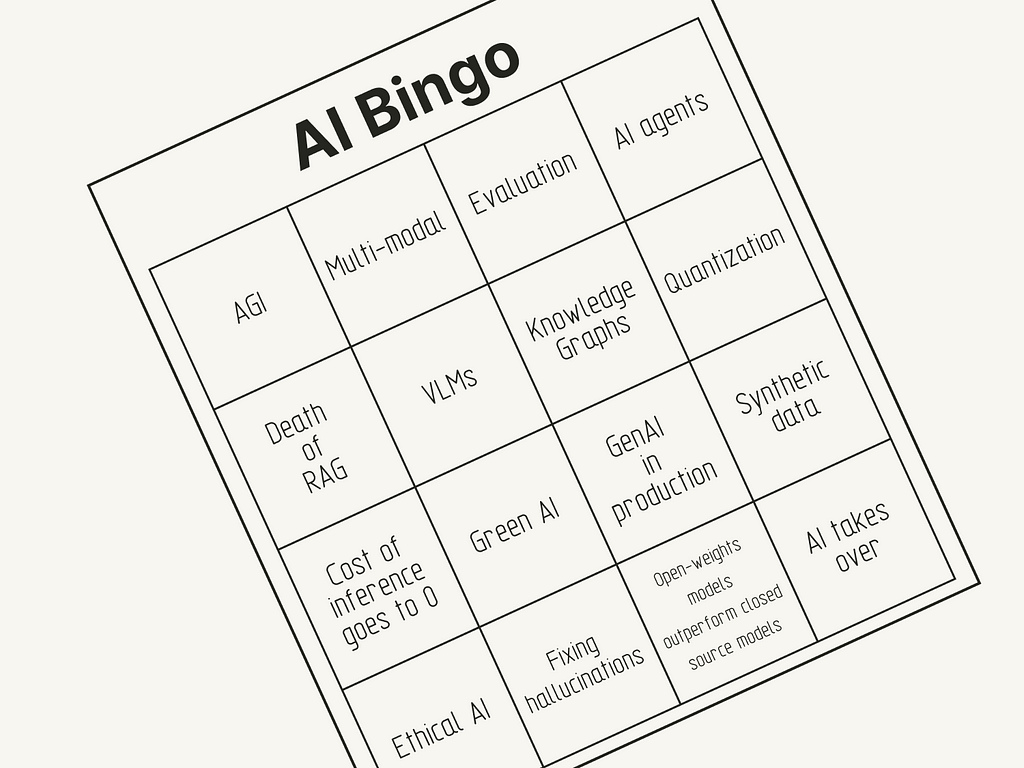
AI Buzzword and Trend Bingo (Image by the author)
In 2023, building AI-powered applications felt full of promise, but the challenges were already starting to show. By 2024, we began experimenting with techniques to tackle the hard realities of making them work in production.
If I have to summarize the AI space in 2024, it would be the “Captain, it’s Wednesday” meme. The amount of major releases this year was overwhelming. I don’t blame anyone in this space who’s feeling exhausted towards the end of this year. It’s been a crazy ride, and it’s been hard to keep up. Let’s review key themes in the AI space and see if I correctly predicted them last year.
Evaluations
Let’s start by looking at some generative AI solutions that made it to production. There aren’t many. As a survey by A16Z revealed in 2024, companies are still hesitant to deploy generative AI in customer-facing applications. Instead, they feel more confident using it for internal tasks, like document search or chatbots.
So, why aren’t there that many customer-facing generative AI applications in the wild? Probably because we are still figuring out how to evaluate them properly. This was one of my predictions for 2024.
Much of the research involved using another LLM to evaluate the output of an LLM (LLM-as-a-judge). While the approach may be clever, it’s also imperfect due to added cost, introduction of bias, and unreliability.
Looking back, I anticipated we would see this issue solved this year. However, looking at the landscape today, despite being a major topic of discussion, we still haven’t found a reliable way to evaluate generative AI solutions effectively. Although I think LLM-as-a-judge is the only way we’re able to evaluate generative AI solutions at scale, this shows how early we are in this field.
Multimodality
Although this one might have been obvious to many of you, I didn’t have this on my radar for 2024. With the releases of GPT4, Llama 3.2, and ColPali, multimodal foundation models were a big trend in 2024. While we, developers, were busy figuring out how to make LLMs work in our existing pipelines, researchers were already one step ahead. They were already building foundation models that could handle more than one modality.
“There is *absolutely no way in hell* we will ever reach human-level AI without getting machines to learn from high-bandwidth sensory inputs, such as vision.” — Yann LeCun
Take PDF parsing as an example of multimodal models’ usefulness beyond text-to-image tasks. ColPali’s researchers avoided the difficult steps of OCR and layout extraction by using visual language models (VLMs). Systems like ColPali and ColQwen2 process PDFs as images, extracting information directly without pre-processing or chunking. This is a reminder that simpler solutions often come from changing how you frame the problem.
Multimodal models are a bigger shift than they might seem. Document search across PDFs is just the beginning. Multimodality in foundation models will unlock entirely new possibilities for applications across industries. With more modalities, AI is no longer just about language — it’s about understanding the world.
Fine-tuning open-weight models and quantization
Open-weight models are closing the performance gap to closed models. Fine-tuning them gives you a performance boost while still being lightweight. Quantization makes these models smaller and more efficient (see also Green AI) to run anywhere, even on small devices. Quantization pairs well with fine-tuning, especially since fine-tuning language models is inherently challenging (see QLoRA).
Together, these trends make it clear that the future isn’t just bigger models — it’s smarter ones.
This year, AI agents and agentic workflows gained much attention, as Andrew Ng predicted at the beginning of the year. We saw Langchain and LlamaIndex move into incorporating agents, CrewAI gained a lot of momentum, and OpenAI came out with Swarm. This is another topic I hadn’t seen coming since I didn’t look into it.
“I think AI agentic workflows will drive massive AI progress this year — perhaps even more than the next generation of foundation models.” — Andrew Ng
Despite the massive interest in AI agents, they can be controversial. First, there is still no clear definition of “AI agent” and its capabilities. Are AI agents just LLMs with access to tools, or do they have other specific capabilities? Second, they come with added latency and cost. I have read many comments saying that agent systems aren’t suitable for production systems due to this.
But I think we have already been seeing some agentic pipelines in production with lightweight workflows, such as routing user queries to specific function calls. I think we will continue to see agents in 2025. Hopefully, we will get a clearer definition and picture.
RAG isn’t de*d and retrieval goes mainstream
Retrieval-Augmented Generation (RAG) gained significant attention in 2023 and remained a key topic in 2024, with many new variants emerging. However, it remains a topic of debate. Some argue it’s becoming obsolete with long-context models, while others question whether it’s even a new idea. While I think the criticism of the terminology is justified, I think the concept is here to stay (for a little while at least).
Every time a new long context model is released, some people predict it will be the end of RAG pipelines. I don’t think that’s going to happen. This whole discussion should be a blog post of its own, so I’m not going into depth here and saving the discussion for another one. Let me just say that I don’t think it’s one or the other. They are complements. Instead, we will probably be using long context models together with RAG pipelines.
Also, having a database in applications is not a new concept. The term ‘RAG,’ which refers to retrieving information from a knowledge source to enhance an LLM’s output, has faced criticism. Some argue it’s merely a rebranding of techniques long used in other fields, such as software engineering. While I think we will probably part from the term in the long run, the technique is here to stay.
Despite predictions of RAG’s demise, retrieval remains a cornerstone of AI pipelines. While I may be biased by my work in retrieval, it felt like this topic became more mainstream in AI this year. It started with many discussions around keyword search (BM25) as a baseline for RAG pipelines. It then evolved into a larger discussion around dense retrieval models, such as ColBERT or ColPali.
Knowledge graphs
I completely missed this topic because I’m not too familiar with it. Knowledge graphs in RAG systems (e.g., Graph RAG) were another big topic. Since all I can say about knowledge graphs at this moment is that they seem to be a powerful external knowledge source, I will keep this section short.
The key topics of 2024 suggest that we are now realizing the limitations of building applications with foundation models. The hype around ChatGPT may have settled, but the drive to integrate foundation models into applications is still very much alive. It’s just way more difficult than we had anticipated.
“ The race to make AI more efficient and more useful, before investors lose their enthusiasm, is on.” — The Economist
2024 taught us that scaling foundation models isn’t enough. We need better evaluation, smarter retrieval, and more efficient workflows to make AI useful. The limitations we ran into this year aren’t signs of stagnation — they’re clues about what we need to fix next in 2025.
My 2025 Predictions
OK, now, for the interesting part, what are my 2025 predictions? This year, I want to make some bolder predictions for the next year to make it a little more fun:
Video will be an important modality: After text-only LLMs evolved into multimodal foundation models (mostly text and images), it’s only natural that video will be the next modality. I can imagine seeing more video-capable foundation models follow in Sora’s footsteps.
From one-shot to agentic to human-in-the-loop: I imagine we will start incorporating humans into AI-powered systems. While we started with one-shot systems, we are not at the stage of having AI agents coordinate different tasks to improve results. But AI agents won’t replace humans. They’ll empower them. Systems that incorporate human feedback will deliver better outcomes across industries. In the long-term, I imagine that we will have to have systems that wait for human feedback before taking action on the next task.
Latency and cost per token will drop: Currently, one big issue for AI agents is added latency and cost. However, with Moore’s law and research for making AI models more efficient, like quantization and efficient training techniques (not only for cost reasons but also for environmental reasons), I can imagine both the latency and cost per token going down.
I am curious to hear your predictions for the AI space in 2025!
PS: Funnily, I was researching recipes for Christmas cookies with ChatGPT a few days ago instead of using Google, which I was wondering about two years ago when ChatGPT was released.
Amazon Bedrock Data Automation in public preview, offers a unified experience for developers of all skillsets to easily automate the extraction, transformation, and generation of relevant insights from documents, images, audio, and videos to build generative AI–powered applications. In this post, we demonstrate how to use Amazon Bedrock Data Automation in the AWS Management Console and the AWS SDK for Python (Boto3) for media analysis and intelligent document processing (IDP) workflows.
Tracking a ball trajectory and visualizing it’s vertical position in real-time animated plots
In Computer Vision a fundamental goal is to extract meaningful information from static images or video sequences. To understand these signals, it is often helpful to visualize them.
For example when tracking individual cars on a highway, we could draw bounding boxes around them or in the case of detecting problems in a product line on a conveyor belt, we could use a distinct color for anomalies. But what if the extracted information is of a more numerical nature and you want to visualize the time dynamics of this signal?
Just showing the value as a number on the screen might not give you enough insight, especially when the signal is changing rapidly. In these cases a great way to visualize the signal is a plot with a time axis. In this post I am going to show you how you can combine the power of OpenCV and Matplotlib to create animated real-time visualizations of such signals.
The code and video I used for this project is available on GitHub:
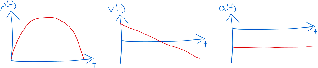
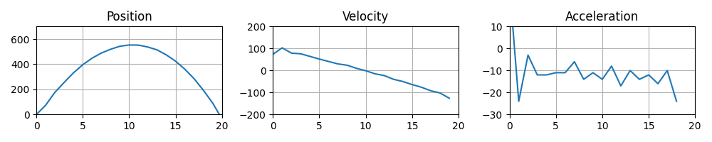
Let’s explore a toy problem where I recorded a video of a ball thrown vertically into the air. The goal is to track the ball in the video and plot it’s position p(t), velocity v(t)and acceleration a(t)over time.
Input Video
Let’s define our reference frame to be the camera and for simplicity we only track the vertical position of the ball in the image. We expect the position to be a parabola, the velocity to linearly decrease and the acceleration to be constant.
Sketch of graphs we should expect
Ball Segmentation
In a first step we need to identify the ball in each frame of the video sequence. Since the camera remains static, an easy way to detect the ball is using a background subtraction model, combined with a color model to remove the hand in the frame.
First let’s get our video clip displayed with a simple loop using VideoCapture from OpenCV. We simply restart the video clip once it has reached its end. We also make sure to playback the video at the original frame rate by calculating the sleep_time in milliseconds based on the FPS of the video. Also make sure to release the resources at the end and close the windows.
import cv2
cap = cv2.VideoCapture("ball.mp4") fps = int(cap.get(cv2.CAP_PROP_FPS))
while True: ret, frame = cap.read() if not ret: cap.set(cv2.CAP_PROP_POS_FRAMES, 0) continue
Let’s first work on extracting a binary segmentation mask for the ball. This essentially means that we want to create a mask that is active for pixels of the ball and inactive for all other pixels. To do this, I will combine two masks: a motion mask and a color mask. The motion mask extracts the moving parts and the color mask mainly gets rid of the hand in the frame.
For the color filter, we can convert the image to the HSV color space and select a specific hue range (20–100) that contains the green colors of the ball but no skin color tones. I don’t filter on the saturation or brightness values, so we can use the full range (0–255).
# filter based on color
hsv = cv2.cvtColor(frame, cv2.COLOR_BGR2HSV)
mask_color = cv2.inRange(hsv, (20, 0, 0), (100, 255, 255))
To create a motion mask we can use a simple background subtraction model. We use the first frame of the video for the background by setting the learning rate to 1. In the loop, we apply the background model to get the foreground mask, but don’t integrate new frames into it by setting the learning rate to 0.
...

# initialize background model
bg_sub = cv2.createBackgroundSubtractorMOG2(varThreshold=50, detectShadows=False)
ret, frame0 = cap.read()
if not ret:
    print("Error: cannot read video file")
    exit(1)
bg_sub.apply(frame0, learningRate=1.0)

while True:
  ...
  # filter based on motion
  mask_fg = bg_sub.apply(frame, learningRate=0)
In the next step, we can combine the two masks and apply a opening morphologyto get rid of the small noise and we end up with a perfect segmentation of the ball.
Top Left: Video Sequence, Top Right: Color Mask, Bottom Left: Motion Mask, Bottom Right: Combined Mask
Tracking the Ball
The only thing we’re left with is our ball in the mask. To track the center of the ball, I first extract the contour of the ball and then take the center of its bounding box as reference point. In case some noise would make it through our mask, I am filtering the detected contours by size and only look at the largest one.
# find largest contour corresponding to the ball we want to track
contours, _ = cv2.findContours(mask, cv2.RETR_EXTERNAL, cv2.CHAIN_APPROX_SIMPLE)
if len(contours) > 0:
    largest_contour = max(contours, key=cv2.contourArea)
    x, y, w, h = cv2.boundingRect(largest_contour)
    center = (x + w // 2, y + h // 2)
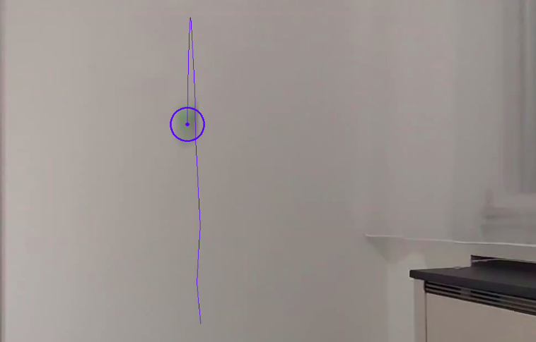
We can also add some annotations to our frame to visualize our detection. I am going to draw two circles, one for the center and one for the perimeter of the ball.
cv2.circle(frame, center, 30, (255, 0, 0), 2)
cv2.circle(frame, center, 2, (255, 0, 0), 2)
To keep track of the ball position, we can use a list. Whenever we detect the ball, we simply add the center position to the list. We can also visualize the trajectory by drawing lines between each of the segments in the tracked position list.
tracked_pos = []


while True:
  ...

  if len(contours) > 0:
    ...
    tracked_pos.append(center)


  # draw trajectory
  for i in range(1, len(tracked_pos)):
      cv2.line(frame, tracked_pos[i - 1], tracked_pos[i], (255, 0, 0), 1)
Visualization of the Ball Trajectory
Creating the Plot
Now that we can track the ball, let’s start exploring how we can plot the signal using matplotlib. In a first step, we can create the final plot at the end of our video first and then in a second step we worry about how to animate it in real-time. To show the position, velocity and acceleration we can use three horizontally aligned subplots:
Static Plots of the Position, Velocity and Acceleration
Animating the Plot
Now on to the fun part, we want to make this plot dynamic! Since we are working in an OpenCV GUI loop, we cannot directly use the show function from matplotlib, as this will just block the loop and not run our program. Instead we need to make use of some trickery ✨
The main idea is to draw the plots in memory into a buffer and then display this buffer in our OpenCV window. By manually calling the draw function of the canvas, we can force the figure to be rendered to a buffer. We can then get this buffer and convert it to an array. Since the buffer is in RGB format, but OpenCV uses BGR, we need to convert the color order.
Now we can simply display the plot using the imshow function from OpenCV.
cv2.imshow("Plot", plot)
Animated Plots
And voilà, you get your animated plot! However you will notice that the performance is quite low. Re-drawing the full plot every frame is quite expensive. To improve the performance, we need to make use of blitting. This is an advanced rendering technique, that draws static parts of the plot into a background image and only re-draws the changing foreground elements. To set this up, we first need to define a reference to each of our three plots before the frame loop.
Then we need to draw the background of the figure once before the loop and get the background of each axis.
fig.canvas.draw()
bg_axs = [fig.canvas.copy_from_bbox(ax.bbox) for ax in axs]
In the loop, we can now change the data for each of the plots and then for each subplot we need to restore the region’s background, draw the new plot and then call the blit function to apply the changes.
# Update plot data pl_pos.set_data(range(len(pos)), pos) pl_vel.set_data(range(len(vel)), vel) pl_acc.set_data(range(len(acc)), acc)
And here we go, the plotting is sped up and the performance has drastically improved.
Optimized Plots
Conclusion
In this post, you learned how to apply simple Computer Vision techniques to extract a moving foreground object and track it’s trajectory. We then created an animated plot using matplotlib and OpenCV. The plotting is demonstrated on a toy example video with a ball being thrown vertically into the air. However, the tools and techniques used in this project are useful for all kinds of tasks and real-world applications! The full source code is available from my GitHub. I hope you learned something today, happy coding and take care!
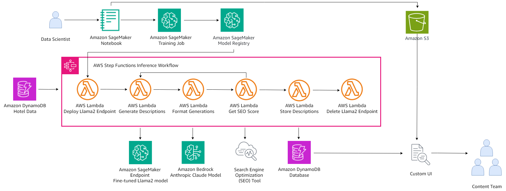
TUI Group is one of the world’s leading global tourism services, providing 21 million customers with an unmatched holiday experience in 180 regions. The TUI content teams are tasked with producing high-quality content for its websites, including product details, hotel information, and travel guides, often using descriptions written by hotel and third-party partners. In this post, we discuss how we used Amazon SageMaker and Amazon Bedrock to build a content generator that rewrites marketing content following specific brand and style guidelines.
Before you start panicking: no, people can’t steal your credit cards via AirDrop.
Contact sharing via the iPhone
Yet another TikTok conspiracy video surrounding the iPhone has taken off. This time, the rumor warns users that AirDrop could be used to give anyone unrestricted access to “everything” stored within your iPhone — including anything stored within Apple Wallet.
It’s unclear what the source of the rumor is, but creators like @vanessaromito13 are directing users to head to settings to disable AirDrop sharing.
We use cookies on our website to give you the most relevant experience by remembering your preferences and repeat visits. By clicking “Accept”, you consent to the use of ALL the cookies.
This website uses cookies to improve your experience while you navigate through the website. Out of these, the cookies that are categorized as necessary are stored on your browser as they are essential for the working of basic functionalities of the website. We also use third-party cookies that help us analyze and understand how you use this website. These cookies will be stored in your browser only with your consent. You also have the option to opt-out of these cookies. But opting out of some of these cookies may affect your browsing experience.
Necessary cookies are absolutely essential for the website to function properly. These cookies ensure basic functionalities and security features of the website, anonymously.
Cookie
Duration
Description
cookielawinfo-checkbox-analytics
11 months
This cookie is set by GDPR Cookie Consent plugin. The cookie is used to store the user consent for the cookies in the category "Analytics".
cookielawinfo-checkbox-functional
11 months
The cookie is set by GDPR cookie consent to record the user consent for the cookies in the category "Functional".
cookielawinfo-checkbox-necessary
11 months
This cookie is set by GDPR Cookie Consent plugin. The cookies is used to store the user consent for the cookies in the category "Necessary".
cookielawinfo-checkbox-others
11 months
This cookie is set by GDPR Cookie Consent plugin. The cookie is used to store the user consent for the cookies in the category "Other.
cookielawinfo-checkbox-performance
11 months
This cookie is set by GDPR Cookie Consent plugin. The cookie is used to store the user consent for the cookies in the category "Performance".
viewed_cookie_policy
11 months
The cookie is set by the GDPR Cookie Consent plugin and is used to store whether or not user has consented to the use of cookies. It does not store any personal data.
Functional cookies help to perform certain functionalities like sharing the content of the website on social media platforms, collect feedbacks, and other third-party features.
Performance cookies are used to understand and analyze the key performance indexes of the website which helps in delivering a better user experience for the visitors.
Analytical cookies are used to understand how visitors interact with the website. These cookies help provide information on metrics the number of visitors, bounce rate, traffic source, etc.
Advertisement cookies are used to provide visitors with relevant ads and marketing campaigns. These cookies track visitors across websites and collect information to provide customized ads.