Tag: tech

A hands-on tutorial in Python for sensor engineers

With contributions from Moritz Berger.

Bayesian sensor calibration is an emerging technique combining statistical models and data to optimally calibrate sensors — a crucial engineering procedure. This tutorial provides the Python code to perform such calibration numerically using existing libraries with a minimal math background. As an example case study, we consider a magnetic field sensor whose sensitivity drifts with temperature.

Glossary. The bolded terms are defined in the International Vocabulary of Metrology (known as the “VIM definitions”). Only the first occurrence is in bold.

Code availability. An executable Jupyter notebook for the tutorial is available on Github. It can be accessed via nbviewer.

Introduction

CONTEXT. Physical sensors provide the primary inputs that enable systems to make sense of their environment. They measure physical quantities such as temperature, electric current, power, speed, or light intensity. A measurement result is an estimate of the true value of the measured quantity (the so-called measurand). Sensors are never perfect. Non-idealities, part-to-part variations, and random noise all contribute to the sensor error. Sensor calibration and the subsequent adjustment are critical steps to minimize sensor measurement uncertainty. The Bayesian approach provides a mathematical framework to represent uncertainty. In particular, how uncertainty is reduced by “smart” calibration combining prior knowledge about past samples and the new evidence provided by the calibration. The math for the exact analytical solution can be intimidating (Berger 2022), even in simple cases where a sensor response is modeled as a polynomial transfer function with noise. Luckily, Python libraries were developed to facilitate Bayesian statistical modeling. Hence, Bayesian models are increasingly accessible to engineers. While hands-on tutorials exist (Copley 2023; Watts 2020) and even textbooks (Davidson-Pilon 2015; Martin 2021), they lack sensor calibration examples.

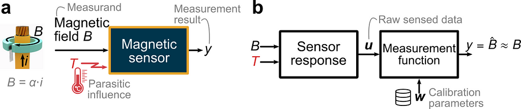
OBJECTIVE. In this article, we aim to reproduce a simplified case inspired by (Berger 2002) and illustrated in the figure below. A sensor is intended to measure the current i flowing through a wire via the measurement of the magnetic field B which is directly proportional to the current. We focus on the magnetic sensor and consider the following non-idealities. (1) The temperature B is a parasitic influence quantity disturbing the measurement. (2) The sensor response varies from one sensor to another due to part-to-part manufacturing variations. (3) The sensed data is polluted by random errors. Using a Bayesian approach and the high-level PyMC Python library, we seek to calculate the optimum set of calibration parameters for a given calibration dataset.

Mathematical formulation

We assume that the magnetic sensor consists of a magnetic and temperature transducer, which can be modeled as polynomial transfer functions with coefficients varying from one sensor to the next according to normal probability distributions. The raw sensed data (called “indications” in the VIM), represented by the vector u, consists of the linearly sensed magnetic field S(T)⋅B and a dimensionless sensed quantity V_T indicative of the temperature. We use the specific form S(T)⋅B to highlight that the sensitivity S is influenced by the temperature. The parasitic influence of the temperature is illustrated by the plot in panel (a) below. Ideally, the sensitivity would be independent of the temperature and of V_T. However, there is a polynomial dependency. The case study being inspired from a real magnetic Hall sensor, the sensitivity can vary by ±40% from its value at room temperature in the temperature range [−40°C, +165°C]. In addition, due to part-to-part variations, there is a set of curves S vs V_T instead of just one curve. Mathematically, we want to identify the measurement function returning an accurate estimate of the true value of the magnetic field — like shown in panel (b). Conceptually, this is equivalent to inverting the sensor response model. This boils down to estimating the temperature-dependent sensitivity and using this estimate Ŝ to recover the field from the sensed field by a division.

For our simplified case, we consider that S(T) and VT(T) are second-order polynomials. The polynomial coefficients are assumed to vary around their nominal values following normal distributions. An extra random noise term is added to both sensed signals. Physically, S is the sensitivity relative to its value at room temperature, and VT is a normalized voltage from a temperature sensor. This is representative of a large class of sensors, where the primary transducer is linear but temperature-dependent, and a supplementary temperature sensor is used to correct the parasitic dependence. And both transducers are noisy. We assume that a third-order polynomial in VT is a suitable candidate for the sensitivity estimate Ŝ:

Ŝ = w_0 + w_1⋅ΔT + w_2⋅ΔT² + w_3⋅ΔT³, where ΔT = T−25°C.

The weight vector w aggregates the 4 coefficients of the polynomial. These are the calibration parameters to be adjusted as a result of calibration.

Python formulation

We use the code convention introduced in (Close, 2021). We define a data dictionary dd to store the nominal value of the parameters. In addition, we define the probability density functions capturing the variability of the parameters. The sensor response is modeled as a transfer function, like the convention introduced in (Close 2021).

# Data dictionary: nominal parameters of the sensor response model
def load_dd():
  return Box({
    'S'  : {
      'TC'   :   [1, -5.26e-3, 15.34e-6],
      'noise':   0.12/100,  },
    'VT': {
      'TC':      [0, 1.16e-3, 2.78e-6],
      'noise':   0.1/100,}  
  })

# Probability density functions for the parameter variations
pdfs = {
    'S.TC': (norm(0,1.132e-2), norm(0,1.23e-4), norm(0,5.40e-7)),
    'VT.TC'   : (norm(0,7.66e-6), norm(0,4.38e-7))
}

# Sensor response model
def sensor_response_model(T, sensor_id=0, dd={}, delta={}):
    S=np.poly1d(np.flip((dd.S.TC+delta.loc[sensor_id]['S.TC'])))(T-25)
    S+=np.random.normal(0, dd.S.noise, size=len(T))
    
    VT = 10*np.poly1d(np.flip(dd.VT.TC+np.r_[0,delta.loc[sensor_id]['VT.TC'].values]))(T-25)
    VT+= np.random.normal(0, dd.VT.noise, size=len(T))
    
    return {'S': S, 'VT': VT}

We can then simulate a first set of N=30 sensors by drawing from the specified probability distributions, and generate synthetic data in df1 to test various calibration approaches via a build function build_sensors(ids=[..]).

df1,_=build_sensors_(ids=np.arange(30))

Classic approaches

We first consider two well-known classic calibration approaches that don’t rely on the Bayesian framework.

Full regression

The first calibration approach is a brute-force approach. A comprehensive dataset is collected for each sensor, with more calibration points than unknowns. The calibration parameters w for each sensor (4 unknowns) are determined by a regression fit. Naturally, this approach provides the best results in terms of residual error. However, it is very costly in practice, as it requires a full characterization of each individual sensor. The following function performs the full calibration and store the weights as a list in the dataframe for convenience.

def full_calibration(df):
    W = df.groupby("id").apply(
        lambda g: ols("S ~ 1 + VT + I(VT**2)+ I(VT**3)", data=g).fit().params
    )
    W.columns = [f"w_{k}" for k, col in enumerate(W.columns)]
    df["w"] = df.apply(lambda X: W.loc[X.name[0]].values, axis=1)

df1, W=full_calibration(df1)

Blind calibration

A blind calibration represents the other extreme. In this approach, a first reference set of sensors is fully calibrated as above. The following sensors are not individually calibrated. Instead, the average calibration parameters w0 of the reference set is reused blindly.

w0 = W.mean().values

df2,_=build_sensors_(ids=[0])
def blind_calibration(df):
    return df.assign(w=[w0]*len(df))
df2 = blind_calibration(df2)

The following plots illustrate the residual sensitivity error Ŝ−S for the two above methods. Recall that the error before calibration reaches up to 40%. The green curves are the sensitivity error for the N=30 sensors from the reference set. Apart from a residual fourth-order error (unavoidable to the limited order of the sensitivity estimator), the fit is satisfactory (<2%). The red curve is the residual sensitivity error for a blindly calibrated sensor. Due to part-to-part variation, the average calibration parameters provide only an approximate fit, and the residual error is not satisfactory.

Bayesian calibration

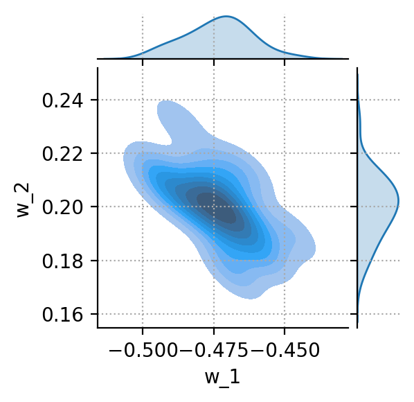
The Bayesian calibration is an interesting trade-off between the previous two extremes. A reference set of sensors is fully calibrated as above. The calibration parameters for this reference set constitute some prior knowledge. The average w0 and the covariance matrix Σ encode some relevant knowledge about the sensor response. The weights are not independent. Some combinations are more probable than others. Such knowledge should be used in a smart calibration. The coverage matrix can be calculated and plotted (for just two weights) using the Pandas and Seaborn libraries.

Cov0 = W.cov(ddof=len(W) - len(w0))
sns.jointplot(data=W.apply(pd.Series),x='w_1', y='w_2', kind='kde', fill=True, height=4)

The Bayesian framework enables us to capture this prior knowledge, and uses it in the calibration of the subsequent samples. We restart from the same blindly calibrated samples above. We simulate the case where just two calibration data points at 0°C and 100°C are collected for each new sensor, enriching our knowledge with new evidence. In practical industrial scenarios where hardware calibration is expensive, this calibration is cost-effective. A reduced reference set is fully characterized once for all to gather prior knowledge. The subsequent samples, possibly the rest of the volume production of this batch, are only characterized at a few points. In Bayesian terminology, this is called “inference”, and the PyMC library provides high-level functions to perform inference. It is a computation-intensive process because the posterior distribution, which is obtained by applying the Bayes’ theorem combining the prior knowledge and the new evidence, can only be sampled. There is no analytical approximation of the obtained probability density function.

The calibration results are compared below, with the blue dot indicating the two calibration points used by the Bayesian approach. With just two extra points and by exploiting the prior knowledge acquired on the reference set, the Bayesian calibrated sensor exhibits an error hardly degraded compared to the expensive brute-force approach.

Credible interval

In the Bayesian approach, all variables are characterized by uncertainty in. The parameters of the sensor model, the calibration parameters, but also the posterior predictions. We can then construct a ±1σ credible interval covering 68% of the synthetic observations generated by the model for the estimated sensitivity Ŝ. This plot captures the essence of the calibration and adjustment: the uncertainty has been reduced around the two calibration points at T=0°C and T=100°C. The residual uncertainty is due to noisy measurements.

Conclusion

This article presented a Python workflow for simulating Bayesian sensor calibration, and compared it against well-known classic approaches. The mathematical and Python formulations are valid for a wide class of sensors, enabling sensor design to explore various approaches. The workflow can be summarized as follows:

1. Model the sensor response in terms of transfer function and the parameters (nominal values and statistical variations). Generate corresponding synthetic raw sensed data for a batch of sensors.
2. Define the form of the measurement function from the raw sensed variables. Typically, this is a polynomial, and the calibration should determine the optimum coefficients w of this polynomial for each sensor.
3. Acquire some prior knowledge by fully characterizing a representative subset of sensors. Encode this knowledge in the form of average calibration parameters and covariance matrix.
4. Acquire limited new evidence in the form of a handful of calibration points specific to each sensor.
5. Perform Bayesian inference merging this new sparse evidence with the prior knowledge to find the most likely calibration parameters for this new sensor numerically using PyMC.

In the frequent cases where sensor calibration is a significant factor of the production cost, Bayesian calibration exhibits substantial business benefits. Consider a batch of 1’000 sensors. One can obtain representative prior knowledge with a full characterization from, say, only 30 sensors. And then for the other 970 sensors, use a few calibration points only. In a classical approach, these extra calibration points lead to an undetermined system of equations. In the Bayesian framework, the prior knowledge fills the gap.

References

(Berger 2022) M. Berger, C. Schott, and O. Paul, “Bayesian sensor calibration,” IEEE Sens. J., 2022. https://doi.org/10.1109/JSEN.2022.3199485.

(Close, 2021): G. Close, “Signal chain analysis in python: a case study for hardware engineers,” Towards Data Science, 22-Feb-2021. Available: https://towardsdatascience.com/signal-chain-analysis-in-python-84513fcf7db2.

(Copley 2023) C. Copley, “Navigating Bayesian Analysis with PyMC,” Towards Data Science, Jun-2023. https://charlescopley.medium.com/navigating-bayesian-analysis-with-pymc-87683c91f3e4

(Davidson-Pilon 2015) C. Davidson-Pilon, “Bayesian Methods for Hackers: Probabilistic Programming and Bayesian Inference,” Addison-Wesley Professional, 2015. https://www.amazon.com/Bayesian-Methods-Hackers-Probabilistic-Addison-Wesley/dp/0133902838

(Martin 2021) O. A. Martin, R. Kumar, and J. Lao, “Bayesian Modeling and Computation in Python,” Chapman and Hall/CRC, 2021. https://www.amazon.com/Bayesian-Modeling-Computation-Chapman-Statistical/dp/036789436X

(Watts 2020) A. Watts, “PyMC3 and Bayesian inference for Parameter Uncertainty Quantification Towards Non-Linear Models: Part 2,” Towards Data Science, Jun-2022. https://towardsdatascience.com/pymc3-and-bayesian-inference-for-parameter-uncertainty-quantification-towards-non-linear-models-a03c3303e6fa

Bayesian Sensor Calibration was originally published in Towards Data Science on Medium, where people are continuing the conversation by highlighting and responding to this story.