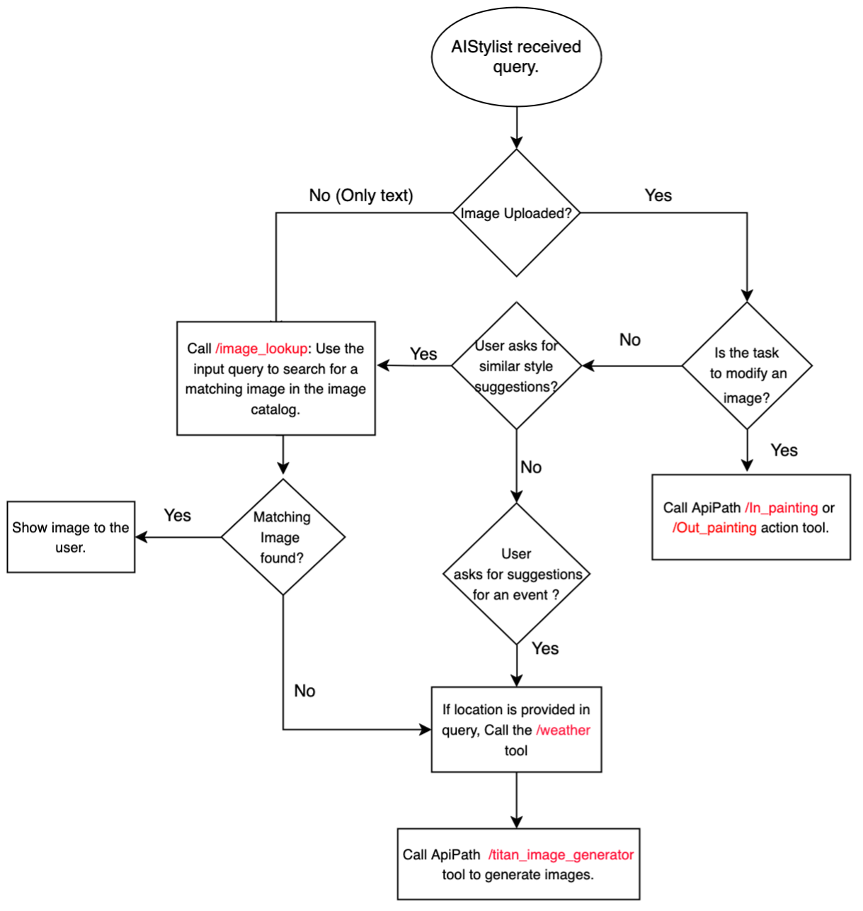
In this post, we implement a fashion assistant agent using Amazon Bedrock Agents and the Amazon Titan family models. The fashion assistant provides a personalized, multimodal conversational experience.
Graphic showing messy data being process. Image by author using ChatGPT-4o.
People use large language models to perform various tasks on text data from different sources. Such tasks may include (but are not limited to) editing, summarizing, translating, or text extraction. One of the primary challenges to this workflow is ensuring your data is AI-ready. This article briefly outlines what AI-ready means and provides a few no-code solutions for getting you to this point.
What does AI-ready mean?
We are surrounded by vast collections of unstructured text data from different sources, including web pages, PDFs, e-mails, organizational documents, etc. In the era of AI, these unstructured text documents can be essential sources of information. For many people, the typical workflow for unstructured text data involves submitting a prompt with a block of text to the large language model (LLM).
Image of a translation task in ChatGPT. Screenshot by author.
While the copy-paste method is a standard strategy for working with LLMs, you will likely encounter situations where this doesn’t work. Consider the following:
While many premium models allow documents to be uploaded and processed, file size is restricted. If the file is too large, you will need other strategies for getting the relevant text into the model.
You may want to process only a small section of text from a larger document. Providing the entire document to the LLM can interfere with the task’s completion because of the irrelevant text.
Some text documents and webpages, especially PDFs, contain a lot of formatting that can interfere with how the text is processed. You may not be able to use the copy-paste method because of how the document is formatted — tables and columns can be problematic.
Being AI-ready means that your data is in a format that can be easily read and processed by an LLM. For text data processing, the data is in plain text with formatting that the LLM readily interprets. The markdown file type is ideal for ensuring your data is AI-ready.
Plain text vs. markdown
Plain text is the most basic type of file on your computer. This is typically denoted as a .txt extension. Many different _editors_ can be used to create and edit plain-text files in the same way that Microsoft Word is used for creating and editing stylized documents. For example, the Notepad application on a PC or the TextEdit application on a Mac are default text editors. However, unlike Microsoft Word, plain-text files do not allow you to stylize the text (e.g., bold, underline, italics, etc.). They are files with only the raw characters in a plain-text format.
Markdown files are plain-text files with the extension .md. What makes the markdown file unique is the use of certain characters to indicate formatting. These special characters are interpreted by Markdown-aware applications to render the text with specific styles and structures. For example, surrounding text with asterisks will be italicized, while double asterisks display the text as bold. Markdown also provides simple ways to create headers, lists, links, and other standard document elements, all while maintaining the file as plain text.
The relationship between Markdown and Large Language Models (LLMs) is straightforward. Markdown files contain plain-text content that LLMs can quickly process and understand. LLMs can recognize and interpret Markdown formatting as meaningful information, enhancing text comprehension. Markdown uses hashtags for headings, which create a hierarchical structure. A single hashtag denotes a level-1 heading, two hashtags a level-2 heading, three hashtags a level-3 heading, and so on. These headings serve as contextual cues for LLMs when processing information. The models can use this structure to understand better the organization and importance of different sections within the text.
By recognizing Markdown elements, LLMs can grasp the content and its intended structure and emphasis. This leads to more accurate interpretation and generation of text. The relationship allows LLMs to extract additional meaning from the text’s structure beyond just the words themselves, enhancing their ability to understand and work with Markdown-formatted documents. In addition, LLMs typically display their output in markdown formatting. So, you can have a much more streamlined workflow working with LLMs by submitting and receiving markdown content. You will also find that many other applications allow for markdown formatting (e.g., Slack, Discord, GitHub, Google Docs)
Many Internet resources exist for learning markdown. Here are a few valuable resources. Please take some time to learn markdown formatting.
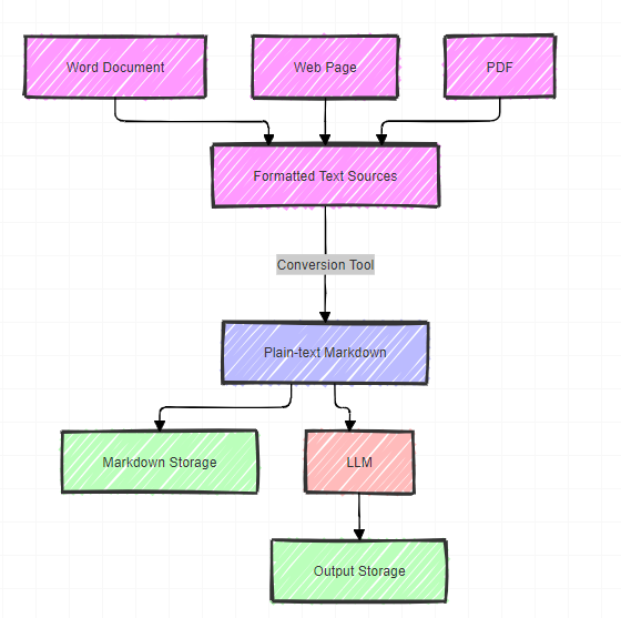
This section explores essential tools for managing Markdown and integrating it with Large Language Models (LLMs). The workflow involves several key steps:
Source Material: We start with structured text sources such as PDFs, web pages, or Word documents.
Conversion: Using specialized tools, we convert these formatted texts into plain text, specifically Markdown format
Storage (Optional): The converted Markdown text can be stored in its original form. This step is recommended if you reuse or reference the text later.
LLM Processing: The Markdown text is then inputted to an LLM.
Output Generation: The LLM processes the data and generates output text.
Result Storage: The LLM’s output can be stored for further use or analysis.
Workflow for converting formatting text to plain text. Image by author using Mermaid diagram.
This workflow efficiently converts various document types into a format that LLMs can quickly process while maintaining the option to store both the input and output for future reference.
Obsidian: Saving and storing plain-text
Obsidian is one of the best options available for saving and storing plain-text and markdown files. When I extract plain-text content from PDFs and web pages, I typically save that content in Obsidian, a free text editor ideal for this purpose. I also use Obsidian for my other work, including taking notes and saving prompts. This is a fantastic tool that is worth learning.
Obsidian is simply a tool for saving and storing plain text content. You will likely want this part of your workflow, but it is NOT required!
Jina AI — Reader: Extract plain text from websites
Jina AI is one of my favorite AI companies. It makes a suite of tools for working with LLMs. Jina AI Reader is a remarkable tool that converts a webpage into markdown format, allowing you to grab content in plain text to be processed by an LLM. The process is very simple. Add https://r.jina.ai/ to any URL, and you will receive AI-ready content for your LLM.
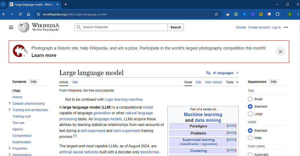
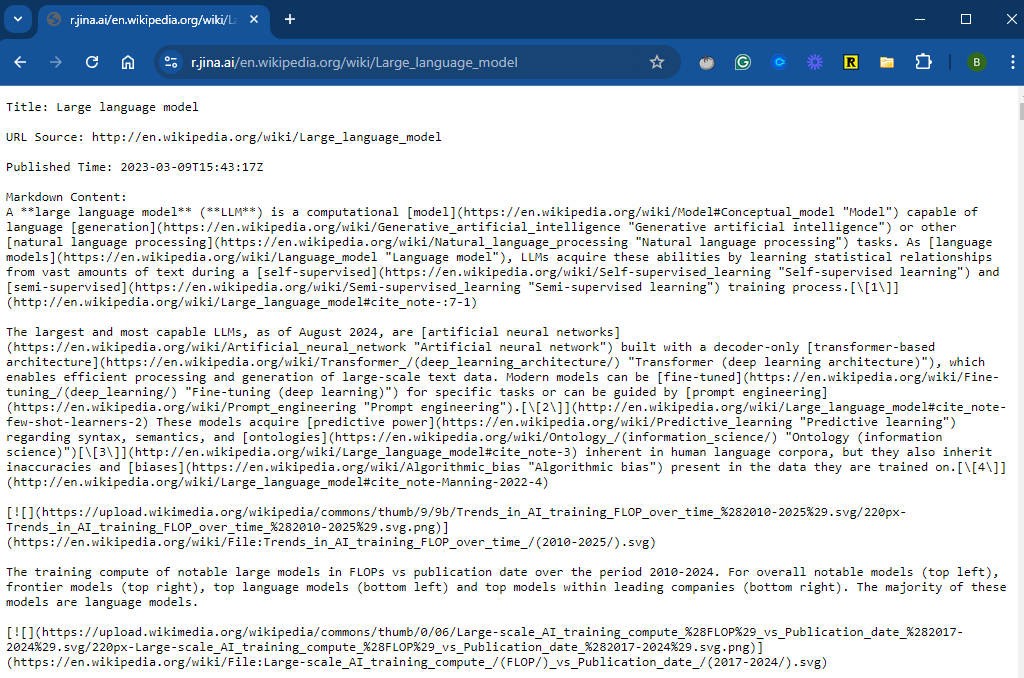
Assume we just wanted to use the text about LLMs contained on this page. Extracting that information can be done using the copy-paste method, but that will be cumbersome with all the other formatting. However, we can use Jina AI-Reader by adding `https://r.jina.ai` to the beginning of the URL:
Wikipedia page converted to markdown via Jina AI-Reader. Image by author.
From here, we can easily copy-paste the relevant content into the LLM. Alternatively, we can save the markdown content in Obsidian, allowing it to be reused over time. While Jina AI offers premium services at a very low cost, you can use this tool for free.
LlamaParse: Extracting plain text from documents
Highly formatted PDFs and other stylized documents present another common challenge. When working with Large Language Models (LLMs), we often must strip away formatting to focus on the content. Consider a scenario where you want to use only specific sections of a PDF report. The document’s complex styling makes simple copy-pasting impractical. Additionally, if you upload the entire document to an LLM, it may struggle to pinpoint and process only the desired sections. This situation calls for a tool that can separate content from formatting. LlamaParse by LlamaIndex addresses this need by effectively decoupling text from its stylistic elements.
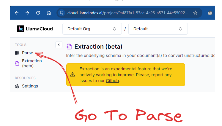
To access LlamaParse, you can log into LlamaCloud: https://cloud.llamaindex.ai/login. After logging into LlamaCloud, go to LlamaParse on the left-hand side of the screen:
Screenshot of LlamaCloud. Image by author.
After you have accessed the Parsing feature, you can extract the content by following these steps. First, change the mode to “Accurate,” which creates output in markdown format. Second, drag and drop your document. You can parse many different types of documents, but my experience is that you will typically need to parse PDFs, Word files, and PowerPoints. Just keep in mind that you can process many different file types. In this example, I use a publicly available report by the American Social Work Board. This is a highly stylized report that is 94 pages long.
Screenshot of LlamaCloud. Image by Author.
Now, you can copy and paste the markdown content or you can export the entire file in markdown.
Screenshot of output from LlamaParse. Image by author.
On the free plan, you can parse 1,000 pages per day. LlamaParse has many other features that are worth exploring.
Final thoughts
Preparing text data for AI analysis involves several strategies. While using these techniques may initially seem challenging, practice will help you become more familiar with the tools and workflows. Over time, you’ll learn to apply them efficiently to your specific tasks.
For several years now, I’ve been dreaming of having a nice portfolio to showcase my projects as a budding data scientist. After almost 1 year of reflection, trials, failures and a few successes, I created my first portfolio on GitHub Pages. Happy with this personal achievement, I wrote an article about it to share the fruit of my research with the community, available here.
This portfolio was created using the mkdocs python package. Mkdocs is a wonderful package for this kind of project, but with a few shortcomings, the main one being the total lack of interactivity with the reader. The further I got into creating my portfolio, the more frustrated I became by the lack of interactivity. My constraints at the time (still true today) were to have everything executed free of charge and client-side, so the GitHub Pages solution was perfectly suited to my needs.
The further I got into my static portfolio, the more the idea of having a dynamic portfolio system popped into my head. My goal was clear: find a solution to create a reader-interactive portfolio hosted on GitHub Pages. In my research, I found almost no articles dealing with this subject, so I started looking for software, packages and code snippets to address this problem.
The research question guiding this article is: how do I create a dynamic, full-client-side website? My technical constraints are as follows: Use GitHub Pages.
About dashboarding package, I choose to limit myself to Panel from the holoviz suite, because it’s a great package and I’d like to improve my skills with it.
For the purposes of this article, I’ve searched for and found many more or less similar solutions. This article is therefore the first in a series of articles, the aim of which will be to present different solutions to the same research question.
But what’s the point of having dynamic Github pages? GitHub Pages is a very interesting solution for organization/project presentation, 100% hosted by GitHub, free of charge, with minimal configuration and no server maintenance. The ability to include dynamic content is a powerful way of communicating about your organization or project. For data professionals, it’s a very useful solution for quickly generating a dynamic and interesting portfolio.
Holoviz is an exciting and extremely rich set of pacakges. It’s a complete visualization and dashboarding solution, powerful on reasonably sized data and big data. This solution supports all major input data manipulation packages (polars, pandas, dask, X-ray, …), and offers high-level syntax for generating interactive visualizations with a minimum of code. This package also allows you to customize the output and, in particular, to choose your visualization back-end such as pandas (I’ve written an article about it if you’d like to find out more). To find out more about this great suite of packages, I suggest this article.
2. Method
For this job, my technical background imposes a few contingencies:
I don’t yet know how to code well enough in JavaScript to make complete scripts and write pieces of code directly in JavaScript,
the dashboarding package will be Panel in order to improve my skills. If the need arises, I won’t rule out repeating the exercise with other dasbhoarding packages (such as Dash, strealint, NiceGUI, etc.). However, this is not my priority.
For this article, my technical environment is as follows:
python packages: Panel
I use conda and VSCode for my scripts and environment management. Don’t worry if you use other solutions, it won’t have any impact on the rest.
During my research, I identified 3 scripts of varying complexity and visual appeal from my researches, which will serve as good test standards:
def add_data(event): b = io.BytesIO() upload.save(b) b.seek(0) name = '.'.join(upload.filename.split('.')[:-1]) select.options[name] = b select.param.trigger('options') select.value = b
widgets = pn.Column( "Select an existing dataset or upload one of your own CSV files and start exploring your data.", pn.Row( select, upload, ) ).servable()
To meet my goal of deploying both web and GitHub Pages, I will test the deployment of each of the :
on a local python server, generated using `python -m http.server`,
GitHub Pages.
Visualize the optimal operation that dasbhoard should have
Before I start testing, I need to have a benchmark of how each application should work in a perfect world. To do this, I use the local emulation function of the :
panel serve simple_app.py --dev
Explanation:
`panel serve simple_app.py` : visualiaze the dashboard
` — dev` : reload the dashboard each time the underlying files are modified (may require installation of one or more other packages, in particular to track whether or not the underlying files have been modified)
Here is the expected result:
The simple app :
Simple app visualization, Image is by the author
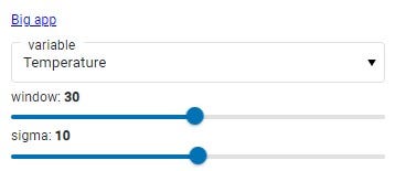
The big app :
Big app visualization, Image is by the author
The material dasbhoard :
Material dashboard visualization, Image is by the author
These visualizations will enable me to see if everything is running smoothly and within reasonable timescales during my deployment tests.
Results
First step : transform python script to HTML interactive script
The Panel package transforms a panel application python script into an HTML application in 1 line of code:
` — to pyodide-worker` : Panel can transcribe the Python application into several types of support that can be integrated into HTML productions. In this article, I focus on the output `pyodide-worker`
` — out docs` : output folder for the 2 files (HTML and JavaScript) generated.
In the docs folder (‘ — to docs’ part of the line of code), 2 files with the same name as the python script and the extensions ‘html’ and ‘js’ should appear. These scripts will enable us to integrate our application into web content. This code conversion (from python to HTML to JavaScript) is made possible by WebAssembly. Pyodide is a port of CPython to WebAssembly/Emscripte (more info here: https://pyodide.org/en/stable/).
If you’re not familiar with WebAssembly, I invite you to devour Mozilla’s article on the subject. I’ll be doing an article on the history, scope and potential impact of WebAssembly, which I think will be a real game changer in the years to come.
First test: local web server deployment
1. Emulate the local web server with python: `python -m http.server`. This command will return a local URL for your browser to connect to (URL like: 127.0.0.1:8000).
2. Click on the HTML script of our python application
Information: when browsing our files via the HTML server, to automatically launch the desired application when we open its folder, title the HTML and JavaScript files ‘index.html’ and ‘index.js’. Example :
app/
|- index.html
|- index.js
When the app folder is opened in the local HTML server, index.html is automatically launched.
Test report for deployment on local html server:
Simple app:✅
Big app:✅
Material Dashboard:✅
After testing each of the 3 applications listed above, this solution works perfectly with all of them, with no loss of speed in loading and using the applications.
Second test: GitHub Pages deployment
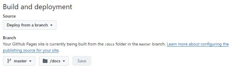
In this article, I’ll quickly go over the configuration part of GitHub Pages on GitHub, as I described it in detail in my previous article.
Warning from step 1: the ‘docs’ file hosting the HTML and JavaScript scripts must be named ‘docs’ and placed at the root of the git repository. These are 2 prerequisites for deploying applications on GitHub Pages. Neither the folder name nor its location can be changed.
2 possibilities : 2.a. Rename the app files ‘index.html’ and ‘index.js’, and place them directly in ‘docs’. This solution will open the GitHub Pages of your repository directly on the app, 2.b. Create an ‘index.html’ file directly in ‘docs’, and add a path to your application’s HTML file.
Here is the content of ‘index.html’ that I created during my deployment tests:
`https://petoulemonde.github.io/`: URL of my portfolio
`article_dynamic_webpages/`: my working repo for this article
`simple_app_pyodide/simple_app.html`: HTML folder/application to open. In the repo, the file is stored in docs/simple_app_pyodide/simple_app.html, but don’t mention ‘docs’ in the absolute path. Why this difference between the file explorer and the link? GitHub deploys from the docs folder, ‘docs’ is its working root.
3. Push in the remote repo (in my previous example, the ‘article_dynamic_webpages’ repo).
4. In the repo, enable the creation of a github project page. In the configuration page, here’s how to configure the GitHub page:
Configuration for deployment on GitHub Pages, Image is by the author
This is where the ‘docs’ folder is essential if we want to deploy our application, otherwise we won’t be able to enter any deployment branches in ‘master’.
Test report: Deployment on GitHub pages:
Simple app: ✅
Big app: ✅
Material dashboard: ✅
Concerning solution 2.b. : This is a particularly interesting solution, as it allows us to have a static home page for our website or portfolio, and then distribute it to special dynamic project pages. It opens the door to both static and dynamic GitHub Pages, using mkdocs for the static aspect and its pretty design, and Panel for the interactive pages. I’ll probably do my next article on this mkdocs + Panel (pyodide-worker) deployment solution, and I’ll be delighted to count you among my readers once again.
Problems encountered
The dashboards tested so far don’t distribute to other pages on the site/portfolio, so the only alternative identified is to create a static home page, which redistributes to dashboards within the site. Is it possible to have a site with several pages without using a static page? The answer is yes, because dasbhaords can themselves integrate links, including links to other dashboards on the same site.
I’ve modified the Material app code to add a link (adding `pn.pane.HTML(…)` ):
pn.template.MaterialTemplate(
  site="Panel",
  title="Getting Started App",
  sidebar=[
    pn.pane.HTML('<a href="127.0.0.1:8000/docs/big_app_pyodide/big_app.html">Big app</a>'), # New line !
    variable_widget,
    window_widget,
    sigma_widget],
  main=[bound_plot],
).servable();
This adds a link to the application’s side bar:
Material dashboard with link visualization, Image is by the author
While the proof here isn’t pretty, it show that a dashboard can integrate links to other pages, so it’s possible to create a site with several pages using Panel alone — brilliant! In fact, I’m concentrating here on the dasbhoarding part of Panel, but Panel can also be used to create static pages, so without even mastering mkdocs, you can create sites with several pages combining static and dynamic elements.
Discussion
Panel is a very interesting and powerful package that lets you create dynamic websites easily and hosted on GitHub Pages, thanks in particular to the magic of WebAssembly. The package really lets you concentrate on creating the dasbhoard, then in just a few lines convert that dasbhoard into web content. Coupled with the ease of use of GitHub Pages, Panel makes it possible to rapidly deploy data dashboards.
This solution, while brilliant, has several limitations that I’ve come across in the course of my testing. The first is that it’s not possible to integrate user-editable and executable code. I’d like to be able to let users explore the data in their own way, by sharing the code I’ve written with them so that they can modify it and explore the data in their own way. The second and final limitation is that customizing dashboards is not as easy as creating them. Hvplot offers, via the explorer tool, a visual solution for exploring data and creating charts. But once in the code, I find customization a little difficult. The packge is awesome in terms of power and functionality, and I’m probably still lacking a bit of skill on it, so I think it’s mainly due to my lack of practice on this package rather than the package itself.
If you’ve made it this far, thank you for your attention! Your comments on my previous article were very helpful. Thanks to you, I’ve discovered Quarto and got some ideas on how to make my articles more interesting for you, the reader. Please leave me a comment to tell me how I could improve my article, both technically and visually, so that I can write an even more interesting article for you next time.
Good luck on your Pythonic adventure! Pierre-Etienne
An inductive bias in machine learning is a constraint on a model given some prior knowledge of the target task. As humans, we can recognize a bird whether it’s flying in the sky or perched in a tree. Moreover, we don’t need to examine every cloud or take in the entirety of the tree to know that we are looking at a bird and not something else. These biases in the vision process are encoded in convolution layers via two properties:
Weight sharing: the same kernel weights are re-used along an input channel’s full width and height.
Locality: the kernel has a much smaller width and height than the input.
We can also encode inductive biases in our choice of input features to the model, which can be interpreted as a constraint on the model itself. Designing input features for a neural network involves a trade-off between expressiveness and inductive bias. On one hand, we want to allow the model the flexibility to learn patterns beyond what we humans can detect and encode. On the other hand, a model without any inductive biases will struggle to learn anything meaningful at all.
In this article, we will explore the inductive biases that go into designing effective position encoders for geographic coordinates. Position on Earth can be a useful input to a wide range of prediction tasks, including image classification. As we will see, using latitude and longitude directly as input features is under-constraining and ultimately will make it harder for the model to learn anything meaningful. Instead, it is more common to encode prior knowledge about latitude and longitude in a nonparametric re-mapping that we call a positional encoder.
Introduction: Position Encoders in Transformers
To motivate the importance of choosing effective position encoder more broadly, let’s first examine the well-known position encoder in the transformer model. We start with the notion that the representation of a token input to an attention block should include some information about its position in the sequence it belongs to. The question is then: how should we encode the position index (0, 1, 2…) into a vector?
Assume we have a position-independent token embedding. One possible approach is to add or concatenate the index value directly to this embedding vector. Here is why this doesn’t work well:
The similarity (dot product) between two embeddings — after their position has been encoded — should be independent of the total number of tokens in the sequence. The two last tokens of a sequence should record the same similarity whether the sequence is 5 or 50 words long.
The similarity between two tokens should not depend on the absolute value of their positions, but only the relative distance between them. Even if the encoded indices were normalized to the range [0, 1], two adjacent tokens at positions 1 and 2 would record a lower similarity than the same two tokens later in the sequence.
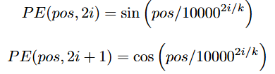
The original “Attention is All You Need” paper [1] proposes instead to encode the position index pos into a discrete “snapshot” of k different sinusoids, where k is the dimension of the token embeddings. These snapshots are computed as follows:
where i = 1, 2, …, k / 2. The resulting k-dimensional position embedding is then added elementwise to the corresponding token embedding.
The intuition behind this encoding is that the more snapshots are out of phase for any two embeddings, the further apart are their corresponding positions. The absolute value of two different positions will not influence how out of phase their snapshots are. Moreover, since the range of any sinusoid is the interval [-1, 1], the magnitude of the positional embeddings will not grow with sequence length.
I won’t go into more detail on this particular position encoder since there are several excellent blog posts that do so (see [2]). Hopefully, you can now see why it is important, in general, to think carefully about how position should be encoded.
Geographic Position Encoders
Let’s now turn to encoders for geographic position. We want to train a neural network to predict some variable of interest given a position on the surface of the Earth. How should we encode a position (λ, ϕ) in spherical coordinates — i.e. a longitude/latitude pair — into a vector that can be used as an input to our network?
One possible approach would be to use latitude and longitude values directly as inputs. In this case our input feature space would be the rectangle [-π, π] × [0, π], which I will refer to as lat/lon space. As with position encoders for transformers, this simple approach unfortunately has its limitations:
Notice that as you move towards the poles, the distance on the surface of the Earth covered by 1 unit of longitude (λ) decreases. Lat/lon space does not preserve distances on the surface of the Earth.
Notice that the position on Earth corresponding to coordinates (λ, ϕ) should be identical to the position corresponding to (λ + 2π, ϕ). But in lat/lon space, these two coordinates are very far apart. Lat/lon space does not preserve periodicity: the way spherical coordinates wrap around the surface of the Earth.
To learn anything meaningful directly from inputs in lat/long space, a neural network must learn how to encode these properties about the curvature of the Earth’s surface on its own — a challenging task. How can we instead design a position encoder that already encodes these inductive biases? Let’s explore some early approaches to this problem and how they have evolved over time.
Early Position Encoders
Discretization-based (2015)
The first paper to propose featurizing geographic coordinates for use as input to a convolutional neural network is called “Improving Image Classification with Location Context” [3]. Published in 2015, this work proposes and evaluates many different featurization approaches with the goal of training better classification models for geo-tagged images.
The idea behind each of their approaches is to directly encode a position on Earth into a set of numerical features that can be computed from auxiliary data sources. Some examples include:
Dividing the U.S. into evenly spaced grids in lat/lon space and using a one-hot encoding to encode a given location into a vector based on which grid it falls into.
Looking up the U.S ZIP code that corresponds to a given location, then retrieving demographic data about this ZIP code from ACS (American Community Survey) related to age, sex, race, living conditions, and more. This is made into a numerical vector using one-hot encodings.
For a chosen set of Instagram hashtags, counting how many hashtags are recorded at different distances from a given location and concatenating these counts into a vector.
Retrieving color-coded maps from Google Maps for various features such as precipitation, land cover, congressional district, and concatenating the numerical color values from each into a vector.
Note that these positional encodings are not continuous and do not preserve distances on the surface of the Earth. In the first example, two nearby locations that fall into different grids will be equally distant in feature space as two locations from opposite sides of the country. Moreover, these features mostly rely on the availability of auxiliary data sources and must be carefully hand-crafted, requiring a specific choice of hashtags, map features, survey data, etc. These approaches do not generalize well to arbitrary locations on Earth.
WRAP (2019)
In 2019, a paper titled “Presence-Only Geographical Priors for Fine-Grained Image Classification” [4] took an important step towards the geographic position encoders commonly used today. Similar to the work from the previous section, this paper studies how to use geographic coordinates for improving image classification models.
The key idea behind their position encoder is to leverage the periodicity of sine and cosine functions to encode the way geographic coordinates wrap around the surface of the Earth. Given latitude and longitude (λ, ϕ), both normalized to the range [-1, 1], the WRAP position encoder is defined as:
Unlike the approaches in the previous section, WRAP is continuous and easily computed for any position on Earth. The paper then shows empirically that training a fully-connected network on top of these features and combining them with latent image features can lead to improved performance on fine-grained image classification benchmarks.
The Double Fourier Sphere Method
The WRAP encoder appears simple, but it successfully encodes a key inductive bias about geographic position while remaining expressive and flexible. In order to see why this choice of position encoder is so powerful, we need to understand the Double Fourier Sphere (DFS) method [5].
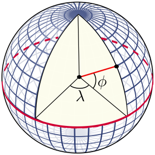
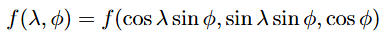
DFS is a method of transforming any real-valued function f (x, y, z) defined on the surface of a unit sphere into a 2π-periodic function defined on a rectangle [-π, π] × [-π, π]. At a high level, DFS consists of two steps:
Re-parametrize the function f (x, y, z) using spherical coordinates, where (λ, ϕ) ∈ [-π, π] × [0, π]
2. Define a new piece-wise function over the rectangle [-π, π] × [-π, π] based on the re-parametrized f (essentially “doubling it over”).
Notice that the DFS re-parametrization of the Earth’s surface (step 1.) preserves the properties we discussed earlier. For one, as ϕ tends to 0 or ± π (the Earth’s poles), the distance between two points (λ, ϕ) and (λ’, ϕ) after re-parametrization decreases. Moreover, the re-parametrization is periodic and smooth.
Fourier Theorem
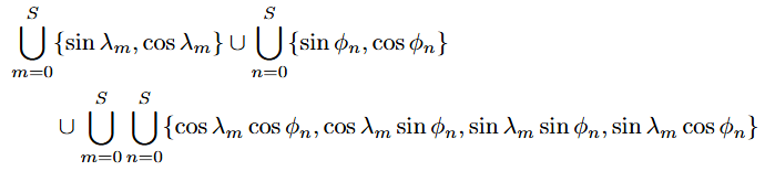
It is a fact that any continuous, periodic, real-valued function can be represented as a weighted sum of sines and cosines. This is called the Fourier Theorem, and this weighted sum representation is called a Fourier series. It turns out that any DFS-transformed function can be represented with a finite set of sines and cosines. They are known as DFS basis functions, listed below:
Here, ∪ denotes union of sets, and S is a collection of scales (i.e. frequencies) for the sinusoids.
DFS-Based Position Encoders
Notice that the set of DFS basis functions includes the four terms in the WRAP position encoder. “Sphere2Vec” [6] is the earliest publication to observe this, proposing a unified view of position encoders based on DFS. In fact, with this generalization in mind, we can construct a geographic position encoder by choosing any subset of the DFS basis functions — WRAP is just one such choice. Take a look at [7] for a comprehensive overview of various DFS-based position encoders.
Why are DFS-based encoders so powerful?
Consider what happens when a linear layer is trained on top of a DFS-based position encoder: each output element of the network is a weighted sum of the chosen DFS basis functions. Hence, the network can be interpreted as a learned Fourier series.Since virtually any function defined on the surface of a sphere can be transformed using the DFS method, it follows that a linear layer trained on top of DFS basis functions is powerful enough to encode arbitrary functions on the sphere! This is akin to the universal approximation theorem for multilayer perceptrons.
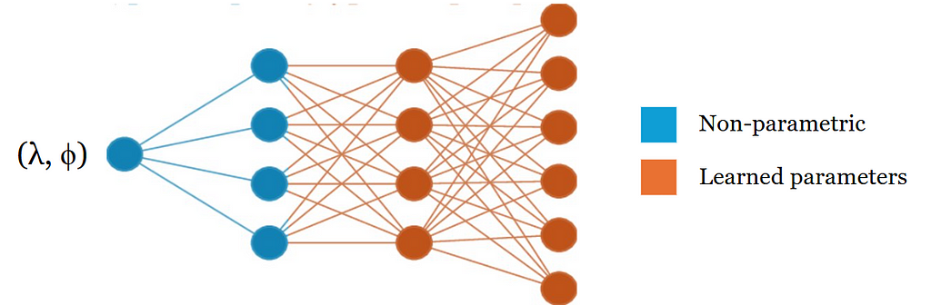
In practice, only a small subset of the DFS basis functions is used for the position encoder and a fully-connected network is trained on top of these. The composition of a non-parametric position encoder with a neural network is commonly referred to as a location encoder:
A depiction of a geographic location encoder. Image by author.
Geographic Location Encoders Today
As we have seen, a DFS-based position encoder can effectively encode inductive biases we have about the curvature of the Earth’s surface. One limitation of DFS-based encoders is that they assume a rectangular domain [-π, π] × [-π, π]. While this is mostly fine since the DFS re-parametrization already accounts for how distances get warped closer to the poles, this assumption breaks down at the poles themselves (ϕ = 0, ± π), which are lines in the rectangular domain that collapse to singular points on the Earth’s surface.
A different set of basis functions called spherical harmonics have recently emerged as an alternative. Spherical harmonics are basis functions that are natively defined on the surface of the sphere as opposed to a rectangle. They have been shown to exhibit fewer artifacts around the Earth’s poles compared to DFS-based encoders [7]. Notably, spherical harmonics are the basis functions used in the SatCLIP location encoder [8], a recent foundation model for geographic coordinates trained in the style of CLIP.
Though geographic position encoders began with discrete, hand-crafted features in the 2010s, these do not easily generalize to arbitrary locations and require domain-specific metadata such as land cover and demographic data. Today, geographic coordinates are much more commonly used as neural network inputs because simple yet meaningful and expressive ways of encoding them have emerged. With the rise of web-scale datasets which are often geo-tagged, the potential for using geographic coordinates as inputs for prediction tasks is now immense.
References
[1] A. Vaswani, N. Shazeer, N. Parmar, J. Uszkoreit, L. Jones, A. N. Gomez, L. Kaiser & I. Polosukhin, Attention Is All You Need (2017), 31st Conference on Neural Information Processing Systems
We use cookies on our website to give you the most relevant experience by remembering your preferences and repeat visits. By clicking “Accept”, you consent to the use of ALL the cookies.
This website uses cookies to improve your experience while you navigate through the website. Out of these, the cookies that are categorized as necessary are stored on your browser as they are essential for the working of basic functionalities of the website. We also use third-party cookies that help us analyze and understand how you use this website. These cookies will be stored in your browser only with your consent. You also have the option to opt-out of these cookies. But opting out of some of these cookies may affect your browsing experience.
Necessary cookies are absolutely essential for the website to function properly. These cookies ensure basic functionalities and security features of the website, anonymously.
Cookie
Duration
Description
cookielawinfo-checkbox-analytics
11 months
This cookie is set by GDPR Cookie Consent plugin. The cookie is used to store the user consent for the cookies in the category "Analytics".
cookielawinfo-checkbox-functional
11 months
The cookie is set by GDPR cookie consent to record the user consent for the cookies in the category "Functional".
cookielawinfo-checkbox-necessary
11 months
This cookie is set by GDPR Cookie Consent plugin. The cookies is used to store the user consent for the cookies in the category "Necessary".
cookielawinfo-checkbox-others
11 months
This cookie is set by GDPR Cookie Consent plugin. The cookie is used to store the user consent for the cookies in the category "Other.
cookielawinfo-checkbox-performance
11 months
This cookie is set by GDPR Cookie Consent plugin. The cookie is used to store the user consent for the cookies in the category "Performance".
viewed_cookie_policy
11 months
The cookie is set by the GDPR Cookie Consent plugin and is used to store whether or not user has consented to the use of cookies. It does not store any personal data.
Functional cookies help to perform certain functionalities like sharing the content of the website on social media platforms, collect feedbacks, and other third-party features.
Performance cookies are used to understand and analyze the key performance indexes of the website which helps in delivering a better user experience for the visitors.
Analytical cookies are used to understand how visitors interact with the website. These cookies help provide information on metrics the number of visitors, bounce rate, traffic source, etc.
Advertisement cookies are used to provide visitors with relevant ads and marketing campaigns. These cookies track visitors across websites and collect information to provide customized ads.