In this post, we present a solution that harnesses the power of generative AI to streamline the user onboarding process for financial services through a digital assistant.
Do you want your Rust code to run everywhere — from large servers to web pages, robots, and even watches? In this second of three articles, I’ll show you how to use WebAssembly (WASM) to run your Rust code directly in the user’s browser.
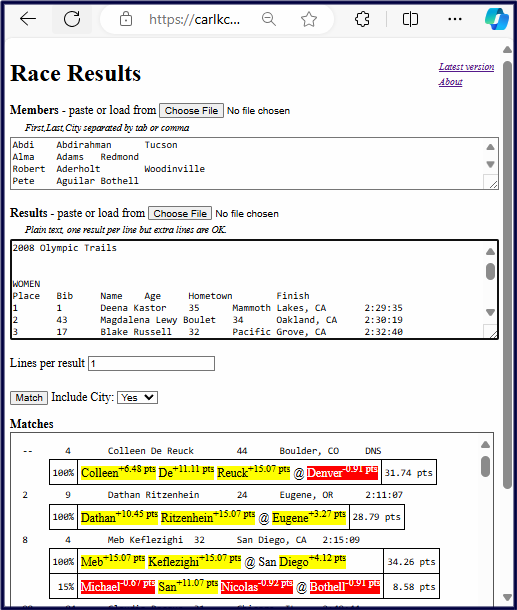
With this technique, you can provide CPU-intensive, dynamic web pages from a — perhaps free — static web server. As a bonus, a user’s data never leaves their machine, avoiding privacy issues. For example, I offer a tool to search race results for friends, running club members, and teammates. To see the tool, go to its web page, and click “match”.
Running Rust in the browser presents challenges. Your code doesn’t have access to a full operating system like Linux, Windows, or macOS. You have no direct access to files or networks. You have only limited access to time and random numbers. We’ll explore workarounds and solutions.
Porting code to WASM in the browser requires several steps and choices, and navigating these can be time-consuming. Missing a step can lead to failure. We’ll reduce this complication by offering nine rules, which we’ll explore in detail:
Confirm that your existing app works with WASM WASI and create a simple JavaScript web page.
Install the wasm32-unknown-unknown target, wasm-pack, wasm-bindgen-cli, and Chrome for Testing & Chromedriver.
Make your project cdylib (and rlib), add wasm-bindgen dependencies, and test.
Learn what types wasm-bindgen supports.
Change functions to use supported types. Change files to generic BufRead.
Adapt tests, skipping those that don’t apply.
Change to JavaScript-friendly dependencies, if necessary. Run tests.
Connect your web page to your functions.
Add wasm-pack to your CI (continuous integration) tests.
Aside: These articles are based on a three-hour workshop that I presented at RustConf24 in Montreal. Thanks to the participants of that workshop. A special thanks, also, to the volunteers from the Seattle Rust Meetup who helped test this material. These articles replace an article I wrote last year with updated information.
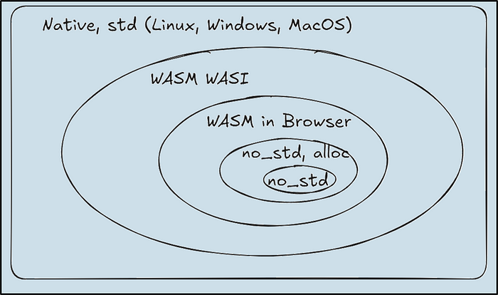
WASM: WebAssembly (WASM) is a binary instruction format that runs in most browsers (and beyond).
WASI: WebAssembly System Interface (WASI) allows outside-the-browser WASM to access file I/O, networking (not yet), and time handling.
no_std: Instructs a Rust program not to use the full standard library, making it suitable for small, embedded devices or highly resource-constrained environments.
alloc: Provides heap memory allocation capabilities (Vec, String, etc.) in no_std environments, essential for dynamically managing memory.
Based on my experience with range-set-blaze, a data structure project, here are the decisions I recommend, described one at a time. To avoid wishy-washiness, I’ll express them as rules.
Rule 1: Confirm that your existing app works with WASM WASI and create a simple JavaScript web page.
Getting your Rust code to run in the browser will be easier if you meet two prerequisites:
Get your Rust code running in WASM WASI.
Get some JavaScript to run in the browser.
For the first prerequisite, see Nine Rules for Running Rust on WASM WASI in Towards Data Science. That article — the first article in this series — details how to move your code from your native operating system to WASM WASI. With that move, you will be halfway to running on WASM in the Browser.
Environments in which we wish to run our code as a Venn diagram of progressively tighter constraints.
Confirm your code runs on WASM WASI via your tests:
For the second prerequisite, show that you can create some JavaScript code and run it in a browser. I suggest adding this index.html file to the top level of your project:
<!DOCTYPE html>
<html lang="en">
<head>
    <meta charset="UTF-8">
    <meta name="viewport" content="width=device-width, initial-scale=1.0">
    <title>Line Counter</title>
</head>
<body>
    <h1>Line Counter</h1>
    <input type="file" id="fileInput" />
    <p id="lineCount">Lines in file: </p>
    <script>
        const output = document.getElementById('lineCount');
        document.getElementById('fileInput').addEventListener('change', (event) => {
            const file = event.target.files[0];
            if (!file) { output.innerHTML = ''; return } // No file selected
            const reader = new FileReader();
            // When the file is fully read
            reader.onload = async (e) => {
                const content = e.target.result;
                const lines = content.split(/rn|n/).length;
                output.textContent = `Lines in file: ${lines}`;
            };
            // Now start to read the file as text
            reader.readAsText(file);
        });
    </script>
</body>
</html>
Now, serve this page to your browser. You can serve web pages via an editor extension. I use Live Preview for VS Code. Alternatively, you can install and use a standalone web server, such as Simple Html Server:
cargo install simple-http-server
simple-http-server --ip 127.0.0.1 --port 3000 --index
# then open browser to http://127.0.0.1:3000
You should now see a web page on which you can select a file. The JavaScript on the page counts the lines in the file.
Let’s go over the key parts of the JavaScript because later we will change it to call Rust.
Aside: Must you learn JavaScript to use Rust in the browser? Yes and no. Yes, you’ll need to create at least some simple JavaScript code. No, you may not need to “learn”JavaScript. I’ve found ChatGPT good enough to generate the simple JavaScript that I need.
See what file the user chose. If none, just return:
const file = event.target.files[0];
if (!file) { output.innerHTML = ''; return } // No file selected
Create a new FileReader object, do some setup, and then read the file as text:
const reader = new FileReader();
// ... some setup ...
// Now start to read the file as text
reader.readAsText(file);
Here is the setup. It says: wait until the file is fully read, read its contents as a string, split the string into lines, and display the number of lines.
// When the file is fully read
reader.onload = async (e) => {
    const content = e.target.result;
    const lines = content.split(/rn|n/).length;
    output.textContent = `Lines in file: ${lines}`;
    };
With the prerequisites fulfilled, we turn next to installing the needed WASM-in-the-Browser tools.
Rule 2: Install the wasm32-unknown-unknown target, wasm-pack, wasm-bindgen-cli, and Chrome for Testing & Chromedriver.
We start with something easy, installing these three tools:
The first line installs a new target, wasm32-unknown-unknown. This target compiles Rust to WebAssembly without any assumptions about the environment the code will run in. The lack of assumptions makes it suitable to run in browsers. (For more on targets, see the previous article’s Rule #2.)
The next two lines install wasm-pack and wasm-bindgen-cli, command-line utilities. The first builds, packages, and publishes into a form suitable for use by a web page. The second makes testing easier. We use –force to ensure the utilities are up-to-date and mutually compatible.
Now, we get to the annoying part, installing Chrome for Testing & Chromedriver. Chrome for Testing is an automatable version of the Chrome browser. Chromedriver is a separate program that can take your Rust tests cases and run them inside Chrome for Testing.
Why is installing them annoying? First, the process is somewhat complex. Second, the version of Chrome for Testing must match the version of Chromedriver. Third, installing Chrome for Testing will conflict with your current installation of regular Chrome.
With that background, here are my suggestions. Start by installing the two programs into a dedicated subfolder of your home directory.
Linux and WSL (Windows Subsystem for Linux):
cd ~
mkdir -p ~/.chrome-for-testing
cd .chrome-for-testing/
wget https://storage.googleapis.com/chrome-for-testing-public/129.0.6668.70/linux64/chrome-linux64.zip
wget https://storage.googleapis.com/chrome-for-testing-public/129.0.6668.70/linux64/chromedriver-linux64.zip
unzip chrome-linux64.zip
unzip chromedriver-linux64.zip
Aside: I’m sorry but I haven’t tested any Mac instructions. Please see the Chrome for Testing web page and then try to adapt the Linux method. If you let me know what works, I’ll update this section.
This installs version 129.0.6668.70, the stable version as of 9/30/2024. If you wish, check the Chrome for Testing Availability page for newer stable versions.
Next, we need to add these programs to our PATH. We can add them temporarily, meaning only for the current terminal session:
# PowerShell
$env:PATH = "$HOME.chrome-for-testingchrome-win64;$HOME.chrome-for-testingchromedriver-win64;$PATH"
# or, CMD
set PATH=%USERPROFILE%.chrome-for-testingchrome-win64;%USERPROFILE%.chrome-for-testingchromedriver-win64;%PATH%
Alternatively, we can add them to our PATH permanently for all future terminal sessions. Understand that this may interfere with access to your regular version of Chrome.
Once installed, you can verify the installation with:
chromedriver --version
Aside: Can you skip installing and using Chrome for Testing and Chromedriver? Yes and no. If you skip them, you’ll still be able to create WASM from your Rust. Moreover, you’ll be able to call that WASM from JavaScript in a web page.
However, your project — like all good code — should already contain tests. If you skip Chrome for Testing, you will not be able to run WASM-in-the-Browser test cases. Moreover, WASM in the Browser violates Rust’s “If it compiles, it works” principle. Specifically, if you use an unsupported feature, like file access, compiling to WASM won’t catch the error. Only test cases can catch such errors. This makes running test cases critically important.
Now that we have the tools to run tests in the browser, let’s try (and almost certainly fail) to run those tests.
Rule 3: Make your project cdylib (and rlib), add wasm-bindgen dependencies, and test.
The wasm-bindgen package is a set of automatically generated bindings between Rust and JavaScript. It lets JavaScript call Rust.
To prepare your code for WASM in the Browser, you’ll make your project a library project. Additionally, you’ll add and use wasm-bindgen dependencies. Follow these steps:
If your project is executable, change it to a library project by renaming src/main.rs to src/lib.rs. Also, comment out your main function.
Make your project create both a static library (the default) and a dynamic library (needed by WASM). Specifically, edit Cargo.toml to include:
Next, what functions do you wish to be visible to JavaScript? Mark those functions with #[wasm_bindgen] and make them pub (public). At the top of the functions’ files, add use wasm_bindgen::prelude::*;.
Aside: For now, your functions may fail to compile. We’ll address this issue in subsequent rules.
What about tests? Everywhere you have a #[test] add a #[wasm_bindgen_test]. Where needed for tests, add this use statement and a configuration statement:
use wasm_bindgen_test::wasm_bindgen_test;
wasm_bindgen_test::wasm_bindgen_test_configure!(run_in_browser);
If you like, you can try the preceding steps on a small, sample project. Install the sample project from GitHub:
# cd to the top of a work directory
git clone --branch native_version --single-branch https://github.com/CarlKCarlK/rustconf24-good-turing.git good-turing
cd good-turing
cargo test
cargo run pg100.txt
Here we see all these changes on the small, sample project’s lib.rs:
// --- May fail to compile for now. ---
use wasm_bindgen::prelude::*;
// ...
#[wasm_bindgen]
pub fn good_turing(file_name: &str) -> Result<(u32, u32), io::Error> {
    let reader = BufReader::new(File::open(file_name)?);
    // ...
}
// fn main() {
// ...
// }
#[cfg(test)]
mod tests {
    use wasm_bindgen_test::wasm_bindgen_test;
    wasm_bindgen_test::wasm_bindgen_test_configure!(run_in_browser);
    // ...
    #[test]
    #[wasm_bindgen_test]
    fn test_process_file() {
      let (prediction, actual) = good_turing("./pg100.txt").unwrap();
      // ...
    }
}
With these changes made, we’re ready to test (and likely fail):
cargo test --target wasm32-unknown-unknown
On this sample, the compiler complains that WASM in the Browser doesn’t like to return tuple types, here, (u32, u32). It also complains that it doesn’t like to return a Result with io::Error. To fix these problems, we’ll need to understand which types WASM in the Browser supports. That’s the topic of Rule 4.
What will happen after we fix the type problems and can run the test? The test will still fail, but now with a runtime error. WASM in the Browser doesn’t support reading from files. The sample test, however, tries to read from a file. In Rule 5, we’ll discuss workarounds for both type limitations and file-access restrictions.
Rule 4: Learn what types wasm-bindgen supports.
Rust functions that JavaScript can see must have input and output types that wasm-bindgen supports. Use of unsupported types causes compiler errors. For example, passing in a u32 is fine. Passing in a tuple of (u32, 32) is not.
More generally, we can sort Rust types into three categories: “Yep!”, “Nope!”, and “Avoid”.
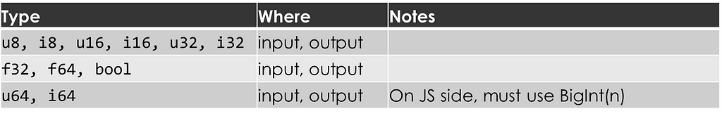
Yep!
This is the category for Rust types that JavaScript (via wasm-bindgen) understands well.
We’ll start with Rust’s simple copy types:
Two items surprised me here. First, 64-bit integers require extra work on the JavaScript side. Specifically, they require the use of JavaScript’s BigInt class. Second, JavaScript does not support 128-bit integers. The 128-bit integers are “Nopes”.
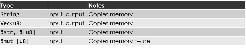
Turning now to String-related and vector-related types:
These super useful types use heap-allocated memory. Because Rust and JavaScript manage memory differently, each language makes its own copy of the data. I thought I might avoid this allocation by passing a &mut [u8] (mutable slice of bytes) from JavaScript to Rust. That didn’t work. Instead of zero copies or one, it copied twice.
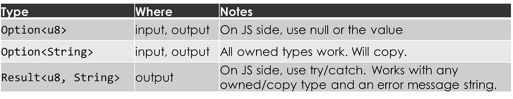
Next, in Rust we love our Option and Result types. I’m happy to report that they are “Yeps”.
A Rust Some(3) becomes a JavaScript 3, and a Rust None becomes a JavaScript null. In other words, wasm-bindgen converts Rust’s type-safe null handling to JavaScript’s old-fashioned approach. In both cases, null/None is handled idiomatically within each language.
Rust Result behaves similarly to Option. A Rust Ok(3) becomes a JavaScript 3, and a Rust Err(“Some error message”) becomes a JavaScript exception that can be caught with try/catch. Note that the value inside the Rust Err is restricted to types that implement the Into<JsValue> trait. Using String generally works well.
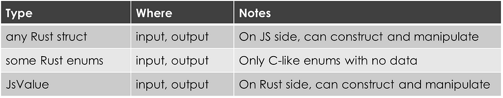
Finally, let’s look at struct, enum, and JSValue, our last set of “Yeps”:
Excitingly, JavaScript can construct and call methods on your Rust structs. To enable this, you need to mark the struct and any JavaScript-accessible methods with #[wasm_bindgen].
For example, suppose you want to avoid passing a giant string from JavaScript to Rust. You could define a Rust struct that processes a series of strings incrementally. JavaScript could construct the struct, feed it chunks from a file, and then ask for the result.
JavaScript’s handling of Rust enums is less exciting. It can only handle enums without associated data (C-like enums) and treats their values as integers.
In the middle of the excitement spectrum, you can pass opaque JavaScript values to Rust as JsValue. Rust can then dynamically inspect the value to determine its subtype or—if applicable—call its methods.
That ends the “Yeps”. Time to look at the “Nopes”.
Nope!
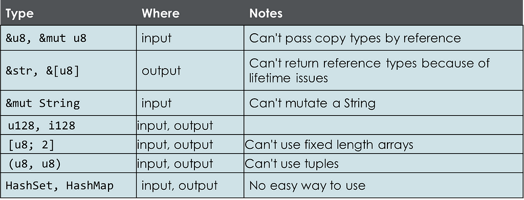
This is the category for Rust types that JavaScript (via wasm-bindgen) doesn’t handle.
Not being able to pass, for example, &u8 by reference is fine because you can just use u8, which is likely more efficient anyway.
Not being able to return a string slice (&str) or a regular slice (&[u8]) is somewhat annoying. To avoid lifetime issues, you must instead return an owned type like String or Vec<u8>.
You can’t accept a mutable String reference (&mut String). However, you can accept a String by value, mutate it, and then return the modified String.
How do we workaround the “Nopes”? In place of fixed-length arrays, tuples, and 128-bit integers, use vectors (Vec<T>) or structs.
Rust has sets and maps. JavaScript has sets and maps. The wasm-bindgen library, however, will not automatically convert between them. So, how can you pass, for example, a HashSet from Rust to JavaScript? Wrap it in your own Rust struct and define needed methods. Then, mark the struct and those methods with #[wasm-bindgen].
And now our third category.
Avoid
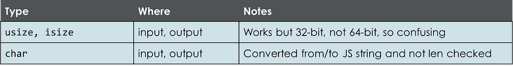
This is the category for Rust types that JavaScript (via wasm-bindgen) allows but that you shouldn’t use.
Avoid using usize and isize because most people will assume they are 64-bit integers, but in WebAssembly (WASM), they are 32-bit integers. Instead, use u32, i32, u64, or i64.
In Rust, char is a special u32 that can contain only valid Unicode scalar values. JavaScript, in contrast, treats a char as a string. It checks for Unicode validity but does not enforce that the string has a length of one. If you need to pass a char from JavaScript into Rust, it’s better to use the String type and then check the length on the Rust side.
Rule 5: Change functions to use supported types. Change files to generic BufRead.
With our knowledge of wasm-bindgen supported types, we can fixup the functions we wish to make available to JavaScript. We left Rule 3’s example with a function like this:
We, now, change the function by removing #[wasm_bindgen] pub. We also change the function to read from a generic reader rather than a file name. Using BufRead allows for more flexibility, enabling the function to accept different types of input streams, such as in-memory data or files.
This wrapper function takes as input a byte slice (&[u8]), something JavaScript can pass. The function turns the byte slice into a reader and calls the inner good_turing. The inner function returns a Result<(u32, u32), io::Error>. The wrapper function translates this result into Result<Vec<u32>, String>, a type that JavaScript will accept.
In general, I’m only willing to make minor changes to functions that will run both natively and in WASM in the Browser. For example, here I’m willing to change the function to work on a generic reader rather than a file name. When JavaScript compatibility requires major, non-idiomatic changes, I create a wrapper function.
In the example, after making these changes, the main code now compiles. The original test, however, does not yet compile. Fixing tests is the topic of Rule 6.
Rule 6: Adapt tests, skipping those that don’t apply.
Rule 3 advocated marking every regular test (#[test]) to also be a WASM-in-the-Browser test (#[wasm_bindgen_test]). However, not all tests from native Rust can be run in a WebAssembly environment, due to WASM’s limitations in accessing system resources like files.
In our example, Rule 3 gives us test code that does not compile:
#[cfg(test)] mod tests { use super::*; use wasm_bindgen_test::wasm_bindgen_test; wasm_bindgen_test::wasm_bindgen_test_configure!(run_in_browser);
This test code fails because our updated good_turing function expects a generic reader rather than a file name. We can fix the test by creating a reader from the sample file:
    use std::fs::File;

    #[test]
    fn test_process_file() {
        let reader = BufReader::new(File::open("pg100.txt").unwrap());
        let (prediction, actual) = good_turing(reader).unwrap();
        assert_eq!(prediction, 10223);
        assert_eq!(actual, 7967);
    }
This is a fine native test. Unfortunately, we can’t run it as a WASM-in-the-Browser test because it uses a file reader — something WASM doesn’t support.
The solution is to create an additional test:
    #[test]
    #[wasm_bindgen_test]
    fn test_good_turing_byte_slice() {
        let data = include_bytes!("../pg100.txt");
        let result = good_turing_byte_slice(data).unwrap();
        assert_eq!(result, vec![10223, 7967]);
    }
At compile time, this test uses the macro include_bytes! to turn a file into a WASM-compatible byte slice. The good_turing_byte_slice function turns the byte slice into a reader and calls good_turing. (The include_bytes macro is part of the Rust standard library and, therefore, available to tests.)
Note that the additional test is both a regular test and a WASM-in-the-Browser test. As much as possible, we want our tests to be both.
In my range-set-blaze project, I was able to mark almost all tests as both regular and WASM in the Browser. One exception: a test used a Criterion benchmarking function. Criterion doesn’t run in WASM in the Browser, so I marked that test regular only (#[test]).
With both our main code (Rule 5) and our test code (Rule 6) fixed, can we actually run our tests? Not necessarily, we may need to find JavaScript friendly dependences.
Aside: If you are on Windows and run WASM-in-the-Browser tests, you may see “ERROR tiny_http] Error accepting new client: A blocking operation was interrupted by a call to WSACancelBlockingCall. (os error 10004)” This is not related to your tests. You may ignore it.
Rule 7: Change to JavaScript-friendly dependencies, if necessary. Run tests.
Dependencies
The sample project will now compile. With my range-set-blaze project, however, fixing my code and tests was not enough. I also needed to fix several dependencies. Specifically, I needed to add this to my Cargo.toml:
[target.'cfg(all(target_arch = "wasm32", target_os = "unknown"))'.dev-dependencies]
getrandom = { version = "0.2", features = ["js"] }
web-time = "1.1.0"
These two dependences enable random numbers and provide an alternative time library. By default, WASM in the Browser has no access to random numbers or time. Both the dependences wrap JavaScript functions making them accessible to and idiomatic for Rust.
Aside: For more information on using cfg expressions in Cargo.toml, see my article: Nine Rust Cargo.toml Wats and Wat Nots: Master Cargo.toml formatting rules and avoid frustration | Towards Data Science (medium.com).
Look for other such JavaScript-wrapping libraries in WebAssembly — Categories — crates.io. Popular crates that I haven’t tried but look interesting include:
Also see Rule 7 in the previous article — about WASM WASI — for more about fixing dependency issues. In the next article in this series — about no_std and embedded — we’ll go deeper into more strategies for fixing dependencies.
Run Tests
With our dependencies fixed, we can finally run our tests, both regular and WASM in the Browser:
cargo test
cargo test --target wasm32-unknown-unknown
Recall that behind the scenes, our call to cargo test –target wasm32-unknown-unknown:
Looks in .cargo/config.toml and sees wasm-bindgen-test-runner (Rule 3).
Calls wasm-bindgen-test-runner.
Uses Chromedriver to run our tests in Chrome for Testing. (Rule 2, be sure Chrome for Testing and Chromedriver are on your path).
With our tests working, we’re now ready to call our Rust code from a web page.
Rule 8: Connect your web page to your functions.
To call your Rust functions from a web page you must first package your Rust library for the web. We installed wasm-pack in Rule 2. Now, we run it:
wasm-pack build --target web
This compiles your project and creates a pkg output directory that JavaScript understands.
Example
In Rule 1, we created an index.html file that didn’t call Rust. Let’s change it now so that it does call Rust. Here is an example of such an index.html followed by a description of the changes of interest.
<script type="module"> import init, { good_turing_byte_slice } from './pkg/good_turing.js'; // These files are generated by `wasm-pack build --target web` const output = document.getElementById('lineCount'); document.getElementById('fileInput').addEventListener('change', (event) => { const file = event.target.files[0]; if (!file) { output.innerHTML = ''; return } // No file selected const reader = new FileReader(); // When the file is fully read reader.onload = async (e) => { await init(); // Ensure 'good_turing_byte_slice' is ready // View the memory buffer as a Uint8Array const u8array = new Uint8Array(e.target.result); try { // Actually run the WASM const [prediction, actual] = good_turing_byte_slice(u8array); output.innerHTML = `Prediction (words that appear exactly once on even lines): ${prediction.toLocaleString()}<br>` + `Actual distinct words that appear only on odd lines: ${actual.toLocaleString()}`; } catch (err) { // Or output an error output.innerHTML = `Error: ${err}`; } }; // Now start to read the file as memory buffer reader.readAsArrayBuffer(file); }); </script> </body> </html>
Let’s go through the changes of interest.
The line below imports two functions into JavaScript from the module file pkg/good_turing.js, which we created using wasm-pack. The default function, init, initializes our Rust-generated WebAssembly (WASM) module. The second function, good_turing_byte_slice, is explicitly imported by including its name in curly brackets.
import init, { good_turing_byte_slice } from './pkg/good_turing.js';
Create a new FileReader object, do some setup, and then read the file as an array of bytes.
const reader = new FileReader();
// ... some setup code ...
// Now start to read the file as bytes.
reader.readAsArrayBuffer(file);
Here is how we setup code that will run after the file is fully read:
reader.onload = async (e) => {
//...
};
This line ensures the WASM module is initialized. The first time it’s called, the module is initialized. On subsequent calls, it does nothing because the module is already ready.
await init(); // Ensure 'good_turing_byte_slice' is ready
Extract the byte array from the read file.
// View the memory buffer as a Uint8Array
const u8array = new Uint8Array(e.target.result);
Aside: Here good_turing_byte_slice is a regular (synchronous) function. If you want, however, you can mark it async on the Rust side and then call it with await on the JavaScript side. If your Rust processing is slow, this can keep your web page more lively.
Display the result.
output.innerHTML =
    `Prediction (words that appear exactly once on even lines): ${prediction.toLocaleString()}<br>` +
    `Actual distinct words that appear only on odd lines: ${actual.toLocaleString()}`;
If there is an error, display the error message.
try { // Actually run the WASM
    // ...
} catch (err) { // Or output an error
    output.innerHTML = `Error: ${err}`;
}
The final code of the sample project is on GitHub, including a README.md that explains what it is doing. Click this link for a live demo.
range-set-blaze
I ported range-set-blaze to WASM at a user’s request so that they could use it inside their own project. The range-set-blaze project is typically used as a library in other projects. In other words, you normally wouldn’t expect range-set-blaze to be the centerpiece of a web page. Nevertheless, I did make a small demo page. You can browse it or inspect its index.html. The page shows how range-set-blaze can turn a list of integers into a sorted list of disjoint ranges.
Aside: Host Your WASM-in-the-Browser Project on GitHub for Free 1. In your project, create a docs folder. 2. Do wasm-pack build –target web. 3. Copy (don’t just move) index.html and pkg into docs. 4. Delete the .gitignore file in docs/pkg. 5. Check the project into GitHub. 6. Go to the project on GitHub. Then go to “Settings”, “Pages”. 7. Set the branch (in my case main) and the folder to docs. Save. 8. The URL will be based on your account and project names, for example, https://carlkcarlk.github.io/rustconf24-good-turing/ 9. To update, repeat steps 2 through 5 (inclusive).
Rule 9: Add wasm-pack to your CI (continuous integration) tests.
Your project is now compiling to WASM in the Browser, passing tests, and showcased on a web page. Are you done? Not quite. Because, as I said in the first article:
If it’s not in CI, it doesn’t exist.
Recall that continuous integration (CI) is a system that can automatically run your tests every time you update your code, ensuring that your code continues to work as expected. In my case, GitHub hosts my project. Here’s the configuration I added to .github/workflows/ci.yml to test my project on WASM in the browser:
  test_wasm_unknown_unknown:
    name: Test WASM unknown unknown
    runs-on: ubuntu-latest
    steps:
      - name: Checkout
        uses: actions/checkout@v4
      - name: Set up Rust
        uses: dtolnay/rust-toolchain@master
        with:
          toolchain: stable
          target: wasm32-unknown-unknown
      - name: Install wasm-pack
        run: |
          curl https://rustwasm.github.io/wasm-pack/installer/init.sh -sSf | sh
      - name: Run WASM tests with Chrome
        run: |
          rustup target add wasm32-unknown-unknown
          wasm-pack test --chrome --headless
By integrating WASM in the Browser into CI, I can confidently add new code to my project. CI will automatically test that all my code continues to support WASM in the browser in the future.
So, there you have it — nine rules for porting your Rust code to WASM in the Browser. Here is what surprised me:
The Bad:
It’s hard to set up testing for WASM in the Browser. Specifically, Chrome for Testing and Chromedriver are hard to install and manage.
WASM in the Browser violates Rust’s saying “If it compiles, it works”. If you use an unsupported feature — for example, direct file access — the compiler won’t catch the error. Instead, you will fail at runtime.
Passing strings and byte vectors creates two copies of your data, one on the JavaScript side and one on the Rust side.
The Good:
WASM in the Browser is useful and fun.
You can mark your regular tests to also run in WASM in the Browser. Just mark your tests with both attributes:
#[test]
#[wasm_bindgen_test]
You can run on WASM in the Browser without needing to port to no_std. Nevertheless, WASM in the Browser is useful as a steppingstone toward running on embedded/no_std.
Stay tuned! In the next article, I’ll show you how to port your Rust code to run in an embedded environment via no_std. This allows your code to run in small devices which I find very cool.
Interested in future articles? Please follow me on Medium. I write about Rust and Python, scientific programming, machine learning, and statistics. I tend to write about one article per month.
Important concepts in information theory, machine learning, and statistics
Image AI-Generated using Gemini
Introduction
In Information Theory, Machine Learning, and Statistics, KL Divergence (Kullback-Leibler Divergence) is a fundamental concept that helps us quantify how two probability distributions differ. It’s often used to measure the amount of information lost when one probability distribution is used to approximate another. This article will explain KL Divergence and some of the other widely used divergences.
KL Divergence
KL Divergence, also known as relative entropy, is a way to measure the difference between two probability distributions, denoted as P and Q. It is often written as —
KL Divergence between two Discrete Distributions P(x) and Q(x)KL Divergence between two Continuous Distributions P(x) and Q(x)
This equation compares the true distribution P with the approximation. distribution Q. Imagine you’re compressing data using an encoding system optimized for one distribution (distribution Q) but the actual data comes from a different distribution (distribution P). KL Divergence measures how inefficient your encoding will be. If Q is close to P, the KL Divergence will be small, meaning less information is lost in the approximation. If Q differs from P, the KL Divergence will be large, indicating significant information loss. In other words, KL Divergence tells you how many extra bits you need to encode data from P when using an encoding scheme designed for Q.
KL Divergence and Shannon’s Entropy
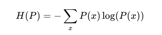
To better understand KL Divergence, it’s useful to relate it to entropy, which measures the uncertainty or randomness of a distribution. The Shannon’s Entropy of a distribution P is defined as:
Shannon Entropy of a distribution P(x)
Recall the popular Binary Cross Entropy Loss function and its curve. Entropy is a measure of uncertainty.
Shannon Entropy Plot (log base is e, can also take base as 2) Pic credit — Author
Entropy tells us how uncertain we are about the outcomes of a random variable. The lower the entropy, the more certain we are about the outcome. The lower the entropy, the more information we have. Entropy is the highest when p=0.5. A probability of 0.5 denotes maximum uncertainty. KL Divergence can be seen as the difference between the entropy of P and the “cross-entropy” between P and Q. Thus, KL Divergence measures the extra uncertainty introduced by using Q instead of P.
Deriving KL Divergence from Entropy
Properties —
KL Divergence is always non-negative.
Proof of non-negativity
Unlike other distance metrics, the KL Divergence is asymmetric.
KL Divergence is asymmetric
Some Applications —
In Variational Auto Encoders, KL Divergence is used as a regularizer to ensure that the latent variable distribution stays close to a prior distribution (typically a standard Gaussian).
KL Divergence quantifies the inefficiency or information loss when using one probability distribution to compress data from another distribution. This is useful in designing and analyzing data compression algorithms.
In reinforcement learning, KL Divergence controls how much a new policy can deviate from an old one during updates. For example, algorithms like Proximal Policy Optimization (PPO) use KL Divergence to constrain policy shifts.
KL Divergence is widely used in industries to detect data drift.
Jensen-Shannon Divergence
Jensen-Shannon Divergence (JS Divergence) is a symmetric measure that quantifies the similarity between two probability distributions. It is based on the KL Divergence. Given two probability distributions P and Q, the Jensen-Shannon Divergence is defined as —
Jenson Shannon Divergence
where M is the average (or mixture) distribution between P and Q.
Mixture Distribution
The first term measures how much information is lost when M is used to approximate P. The second term measures the information loss when M is used to approximate Q. JS Divergence computes the average of the two KL divergences with respect to the average distribution M. KL Divergence penalizes you for using one distribution to approximate another. Still, it is sensitive to which distribution you start from. This asymmetry is often problematic when you want to compare distributions without bias. JS Divergence fixes this by averaging between the two distributions. It doesn’t treat either P or Q as the “correct” distribution but looks at their combined behavior through the mixture distribution M.
Renyi Entropy and Renyi Divergence
We saw earlier that KL Divergence is related to Shannon Entropy. Shannon Entropy is a special case of Renyi Entropy. Renyi Entropy of a distribution is defined as —
Renyi Entropy of a distribution P(x), with parameter α
Renyi Entropy is parameterized by α>0. α controls how much weight is given to different probabilities in the distribution.
α=1: Renyi Entropy equals Shannon Entropy, giving equal weightage to all probable events. You can derive it using limits and the L’Hospital rule.
Deriving Shannon Entropy from Renyi Entropy
α<1: The entropy increases sensitivity to rare events (lower probabilities), making it more focused on the diversity or spread of the distribution.
α>1: The entropy increases sensitivity to common events (higher probabilities), making it more focused on the concentration or dominance of a few outcomes.
Renyi Entropy Plot for different values of α (log base is e, can also take base as 2) Pic credit — Author
α=0: Renyi Entropy approaches the logarithm of the number of possible outcomes (assuming all outcomes are non-zero). This is called the Hartley Entropy.
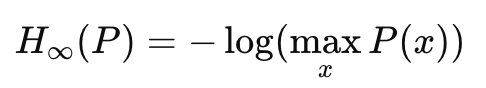
α=∞: As α→∞, Renyi entropy becomes the min-entropy, focusing solely on the most probable outcome.
min-entropy
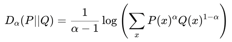
The Renyi Divergence is a metric based on Renyi Entropy. The Renyi Divergence between two distributions P and Q, parameterized by α is defined by —
Renyi Divergence between two Discrete Distributions P(x) and Q(x), with parameter α
KL Divergence is a special case of Renyi Divergence, where α=1.
Deriving KL Divergence from Renyi Divergence
α<1: Focuses on rare events; more sensitive to tail distributions.
α>1: Focuses on common events; more sensitive to high-probability regions.
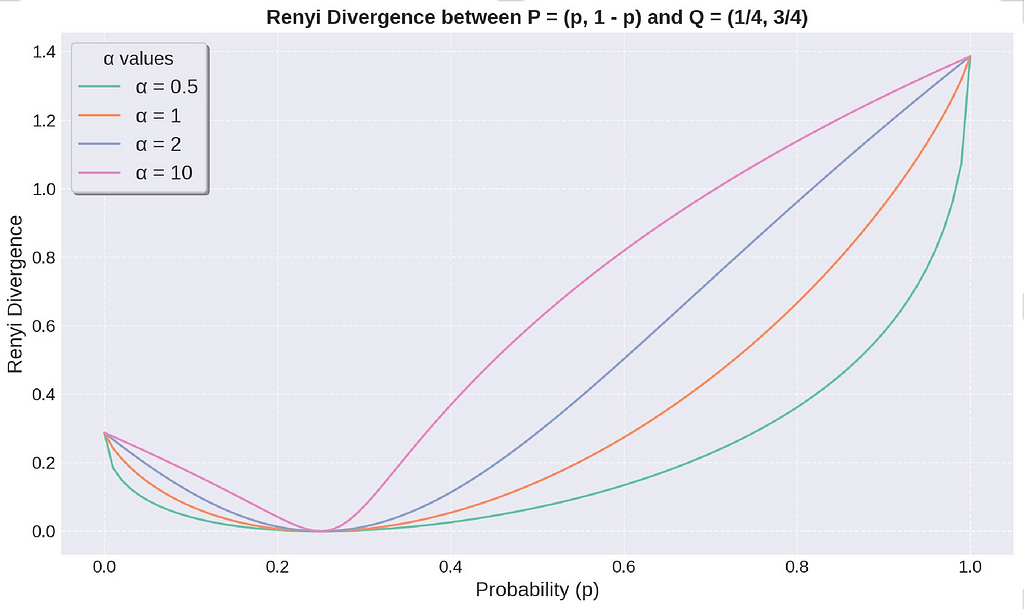
Renyi Divergence Plot between P and Q. Pic credit — Author
The Renyi Divergence is always non-zero and equal to 0 when P = Q. The above figure illustrates how the divergence changes when we vary the distribution P. The divergence increases, with the amount of increase depending on the value of α. A higher value α makes Renyi Divergence more sensitive to changes in probability distribution.
Renyi Divergence finds its application in Differential Privacy, an important concept in Privacy Preserving Machine Learning. Differential Privacy is a mathematical framework that guarantees individuals’ privacy when their data is included in a dataset. It ensures that the output of an algorithm is not significantly affected by the inclusion or exclusion of any single individual’s data. Renyi Differential Privacy (RDP) is an extension of differential privacy that uses Rényi divergence to provide tighter privacy guarantees. We will discuss them in a future blog.
Toy Example — Detecting Data Drift
In an e-commerce setup, data drift can occur when the underlying probability distribution of user behavior changes over time. This can affect various aspects of the business, such as product recommendations. To illustrate how different divergences can be used to detect this drift, consider the following toy example involving customer purchase behavior over seven weeks.
Imagine an e-commerce platform that tracks customer purchases across five product categories: Electronics, Clothing, Books, Home & Kitchen, and Toys. The platform collects click data weekly on the proportion of clicks in each category. These are represented as probability distributions shown in the following code block.
Week 1 to Week 2: There’s a minor drift, with the second category increasing in clicks slightly.
Week 3: A more pronounced drift occurs as the second category becomes more dominant.
Week 5 to Week 7: A significant shift happens where the second category keeps increasing its click share, while others, especially the first category, lose relevance.
We can calculate the divergences using the following—
KL Divergence shows increasing values, indicating that the distribution of purchases diverges more from the baseline as time goes on. From Week 1 to Week 7, KL Divergence emphasizes changes in the second product category, which continues to dominate. Jensen-Shannon Divergence shows a similar smoothly increasing trend, confirming that the distributions are becoming less similar. JS captures the collective drift across the categories.
Renyi Divergence varies significantly based on the chosen α.
With α=0.5, the divergence will place more weight on rare categories (categories 4 and 5 in the distribution). It picks up the drift earlier when these rare categories fluctuate, especially from Week 6 to Week 7 when their probabilities drop to 0.025.
With α=2, the divergence highlights the growing dominance of the second category, showing that high-probability items are shifting and the distribution is becoming less diverse.
You can visualize these trends in the figure above, where you can observe the sharp rise in slopes. By tracking the divergences over the weeks, the e-commerce platform can detect data drift and take measures, such as retraining product recommendation models.
This is the third part of a series of posts on the topic of building custom operators for optimizing AI/ML workloads. In our previous post we demonstrated the simplicity and accessibility of Triton. Named for the Greek god of the sea, Triton empowers Python developers to increase their control over the GPU and optimize its use for the specific workload at hand. In this post we move one step down the lineage of Greek mythology to Triton’s daughter, Pallas and discuss her namesake, the JAX extension for writing custom kernels for GPU and TPU.
One of the most important features of NVIDIA GPUs — and a significant factor in their rise to prominence — is their programmability. A key ingredient of the GPU offering are frameworks for creating General-Purpose GPU (GPGPU) operators, such as CUDA and Triton.
In previous posts (e.g., here) we discussed the opportunity for running ML workloads on Google TPUs and the potential for a meaningful increase in price performance and a reduction in training costs. One of the disadvantages that we noted at the time was the absence of tools for creating custom operators. As a result, models requiring unique operators that were either unsupported by the underlying ML framework (e.g., TensorFlow/XLA) or implemented in a suboptimal manner, would underperform on TPU compared to GPU. This development gap was particularly noticeable over the past few years with the frequent introduction of newer and faster solutions for computing attention on GPU. Enabled by GPU kernel development frameworks, these led to a significant improvement in the efficiency of transformer models.
On TPUs, on the other hand, the lack of appropriate tooling prevented this innovation and transformer models were stuck with the attention mechanisms that were supported by the official SW stack. Fortunately, with the advent of Pallas this gap has been addressed. Built as an extension to JAX and with dedicated support for PyTorch/XLA, Pallas enables the creation of custom kernels for GPU and TPU. For its GPU support Pallas utilizes Triton, and for its TPU support it uses a library called Mosaic. Although we will focus on custom kernels for TPU, it is worth noting that when developing in JAX, GPU kernel customization with Pallas offers some advantages over Triton (e.g., see here).
Our intention in this post is to draw attention to Pallas and demonstrate its potential. Please do not view this post as a replacement for the official Pallas documentation. The examples we will share were chosen for demonstrative purposes, only. We have made no effort to optimize these or verify their robustness, durability, or accuracy.
Importantly, at the time of this writing Pallas is an experimental feature and still under active development. The samples we share (which are based on JAX version 0.4.32 and PyTorch version 2.4.1) may become outdated by the time you read this. Be sure to use the most up-to-date APIs and resources available for your Pallas development.
Many thanks to Yitzhak Levi for his contributions to this post.
Environment Setup
For the experiments described below we use the following environment setup commands:
# check TPU node status (wait for state to be ACTIVE) gcloud alpha compute tpus queued-resources describe v5litepod-1-resource --project <project-id> --zone us-central1-a
In the toy example of our first post in this series, we distinguished between two different ways in which custom kernel development can potentially boost performance. The first is by combining (fusing) together multiple operations in a manner that reduces the overhead of: 1) loading multiple individual kernels, and 2) reading and writing intermediate values (e.g., see PyTorch’s tutorial on multiply-add fusion). The second is by meticulously applying the resources of the underlying accelerator in manner that optimizes the function at hand. We briefly discuss these two opportunities as they pertain to developing custom TPU kernels and make note of the limitations of the Pallas support.
Operator Fusion on TPU
The TPU is an XLA (Accelerated Linear Algebra) device, i.e., it runs code that has been generated by the XLA compiler. When training an AI model in a frameworks such as JAX or PyTorch/XLA, the training step is first transformed into an intermediate graph representation (IR). This computation graph is then fed to the XLA compiler which converts it into machine code that can run on the TPU. Contrary to eager execution mode, in which operations are executed individually, this mode of running models enables XLA to identify and implement opportunities for operator fusion during compilation. And, in fact, operator fusion is the XLA compiler’s most important optimization. Naturally, no compiler is perfect and we are certain to come across additional opportunities for fusion through custom kernels. But, generally speaking, we might expect the opportunity for boosting runtime performance in this manner to be lower than in the case of eager execution.
Optimizing TPU Utilization
Creating optimal kernels for TPU requires a comprehensive and intimate understanding of the TPU system architecture. Importantly, TPUs are very different from GPUs: expertise in GPUs and CUDA does not immediately carry over to TPU development. For example, while GPUs contain a large number of processors and draw their strength from their ability to perform massive parallelization, TPUs are primarily sequential with dedicated engines for running highly vectorized operations and support for asynchronous scheduling and memory loading.
The differences between the underlying architectures of the GPU and TPU can have significant implications on how custom kernels should be designed. Mastering TPU kernel development requires 1) appropriate overlapping of memory and compute operations via pipelining, 2) knowing how to mix between the use of the scalar, vector (VPU) and matrix (MXU) compute units and their associated scalar and vector registers (SREG and VREG) and memory caches (SMEM and VMEM), 3) a comprehension of the costs of different low-level operations, 4) appropriate megacore configuration (on supporting TPU generations), 5) a grasp of the different types of TPU topologies and their implications on how to support distributed computing, and more.
Framework Limitations
While the ability to create custom operators in Python using JAX functions and APIs greatly increases the simplicity and accessibility of Pallas kernel development, it also limits its expressivity. Additionally, (as of the time of this writing) there are some JAX APIs that are not supported by Pallas on TPU (e.g., see here). As a result, you may approach Pallas with the intention of implementing a particular operation only to discover that the framework does not support the APIs that you need. This is in contrast to frameworks such as CUDA which enable a great deal of flexibility when developing custom kernels (for GPU).
The matrix multiplication tutorial in the Pallas documentation provides an excellent introduction to Pallas kernel development, highlighting the potential for operator fusion and customization alongside the challenges involved in optimizing performance (e.g., appropriate tuning of the input block size). The tutorial clearly illustrates that maximizing the full potential of the TPU requires a certain degree of specialization. However, as we intend to demonstrate, even the novice ML developer can benefit from Pallas kernels.
Integrating the Use of Existing Pallas Kernels
To benefit from custom Pallas kernels you do not necessarily need to know how to build them. In our first example we demonstrate how you can leverage existing Pallas kernels from dedicated public repositories.
Example — Flash Attention in Torch/XLA
The JAX github repository includes implementations of a number of Pallas kernels, including flash attention. Here we will demonstrate its use in a Torch/XLA Vision Transformer (ViT) model. Although Pallas kernels are developed in JAX, they can be adopted into Torch/XLA, e.g., via the make_kernel_from_pallas utility (see the documentation for details). In the case of flash attention the adoption is implemented by Torch/XLA.
In the following code block we define a stripped down version of the classic timm attention block with an option to define the underlying attention operator in the constructor. We will use this option to compare the performance of the flash attention Pallas kernel to its alternatives.
# general imports import os, time, functools # torch imports import torch import torch.nn as nn import torch.nn.functional as F from torch.utils.data import Dataset, DataLoader import torch_xla.core.xla_model as xm # custom kernel import from torch_xla.experimental.custom_kernel import flash_attention # timm imports from timm.layers import Mlp from timm.models.vision_transformer import VisionTransformer
# configure the VisionTranformer in a manner that complies with the # Pallas flash_attention kernel constraints model = VisionTransformer( block_fn=functools.partial(TPUAttentionBlock, attn_fn=attn_fn), img_size=256, class_token=False, global_pool="avg" )
# copy the model to the TPU model = model.to(device)
model.train()
t0 = time.perf_counter() summ = 0 count = 0
for step, data in enumerate(train_loader): # copy data to TPU inputs = data[0].to(device=device, non_blocking=True) label = data[1].to(device=device, non_blocking=True)
optimizer.zero_grad(set_to_none=True) with torch.autocast('xla', dtype=torch.bfloat16): output = model(inputs) loss = loss_fn(output, label) loss.backward() optimizer.step() xm.mark_step()
# capture step time batch_time = time.perf_counter() - t0 if step > 20: # skip first steps summ += batch_time count += 1 t0 = time.perf_counter() if step > 100: break
print(f'average step time: {summ / count}')
Note the specific configuration we chose for the VisionTransformer. This is to comply with certain restrictions (as of the time of this writing) of the custom flash attention kernel (e.g., on tensor shapes).
Finally, we define a dataset and compare the runtimes of training with three different attention routines, 1. using native PyTorch functions, 2. using PyTorch’s built in SDPA function, and 3. using the custom Pallas operator:
# use random data class FakeDataset(Dataset): def __len__(self): return 1000000
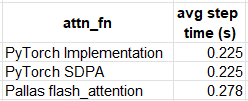
The comparative results are captured in the table below:
Step time for different attention blocks (lower is better) — by Author
Although our Pallas kernel clearly underperforms when compared to its alternatives, we should not be discouraged:
It is likely that these results could be improved with appropriate tuning.
These results are specific to the model and runtime environment that we chose. The Pallas kernel may exhibit wholly different comparative results in other use cases.
The real power of Pallas is in the ability to create and adjust low level operators to our specific needs. Although runtime performance is important, a 23% performance penalty (as in our example) may be a small price to pay for this flexibility. Moreover, the opportunity for customization may open up possibilities for optimizations that are not supported by the native framework operations.
Enhancing Existing Kernels
Oftentimes it may be easier to tweak an existing Pallas kernel to your specific needs, rather than creating one from scratch. This is especially recommended if the kernel has already been optimized as performance tuning can be tedious and time-consuming. The official matrix multiplication tutorial includes a few examples of how to extend and enhance an existing kernel. Here we undertake one of the suggested exercises: we implement int8 matrix multiplication and assess its performance advantage over its bfloat16 alternative.
Example — Int8 Matrix Multiplication
In the code block below we implement an int8 version of the matrix multiplication example.
import functools, timeit import jax import jax.numpy as jnp from jax.experimental import pallas as pl from jax.experimental.pallas import tpu as pltpu
# set to True to develop/debug on CPU interpret = False
@functools.partial(jax.jit, static_argnames=['bm', 'bk', 'bn']) def matmul_int8( x: jax.Array, y: jax.Array, *, bm: int = 128, bk: int = 128, bn: int = 128, ): m, k = x.shape _, n = y.shape return pl.pallas_call( functools.partial(matmul_kernel_int8, nsteps=k // bk), grid_spec=pltpu.PrefetchScalarGridSpec( num_scalar_prefetch=0, in_specs=[ pl.BlockSpec(block_shape=(bm, bk), index_map=lambda i, j, k: (i, k)), pl.BlockSpec(block_shape=(bk, bn), index_map=lambda i, j, k: (k, j)), ], out_specs=pl.BlockSpec(block_shape=(bm, bn), index_map=lambda i, j, k: (i, j)), scratch_shapes=[pltpu.VMEM((bm, bn), jnp.int32)], grid=(m // bm, n // bn, k // bk), ), out_shape=jax.ShapeDtypeStruct((m, n), jnp.int32), compiler_params=dict(mosaic=dict( dimension_semantics=("parallel", "parallel", "arbitrary"))), interpret=interpret )(x, y)
Note our use of an int32 accumulation matrix for addressing the possibility of overflow. Also note our use of the interpretflag for debugging of Pallas kernels on CPU (as recommended here).
To assess our kernel, we introduce a slight modification to the benchmarking utilities defined in the tutorial and compare the runtime results to both the jnp.float16 Pallas matmulkernel and the built-in JAX matmul API:
def benchmark(f, ntrials: int = 100): def run(*args, **kwargs): # Compile function first jax.block_until_ready(f(*args, **kwargs)) # Time function res=timeit.timeit(lambda: jax.block_until_ready(f(*args, **kwargs)), number=ntrials ) time = res/ntrials # print(f"Time: {time}") return time
The results of our experiment are captured in the table below:
Matmul time and utilization (by Author)
By using int8 matrices (rather than bfloat16matrices) on tpuv5e we can boost the runtime performance of our custom matrix multiplication kernel by 71%. However, as in the case of the bfloat16 example, additional tuning is required to match the performance of the built-in matmul operator. The potential for improvement is highlighted by the drop in system utilization when compared to bfloat16.
Creating a Kernel from Scratch
While leveraging existing kernels can be greatly beneficial, it is unlikely to solve all of your problems. Inevitably, you may need to implement an operation that is either unsupported on TPU or exhibits suboptimal performance. Here we demonstrate the creation of a relatively simple pixel-wise kernel. For the sake of continuity, we choose the same Generalized Intersection Over Union (GIOU) operation as in our previous posts.
Example — A GIOU Pallas Kernel
In the code block below we define a Pallas kernel that implements GIOU on pairs of batches of bounding boxes, each of dimension BxNx4 (where we denote the batch size by B and the number of boxes per sample by N). The function returns a tensor of scores of dimension BxN. We choose a block size of 128 on both the batch axis and the boxes axis, i.e., we divide each of the tensors into blocks of 128x128x4 and pass them to our kernel function. The gridand BlockSpec index_map are defined accordingly.
import timeit import jax from jax.experimental import pallas as pl import jax.numpy as jnp
# set to True to develop/debug on CPU interpret = False
# perform giou on a single block def giou_kernel(preds_left_ref, preds_top_ref, preds_right_ref, preds_bottom_ref, targets_left_ref, targets_top_ref, targets_right_ref, targets_bottom_ref, output_ref): epsilon = 1e-5
# copy tensors into local memory preds_left = preds_left_ref[...] preds_top = preds_top_ref[...] preds_right = preds_right_ref[...] preds_bottom = preds_bottom_ref[...]
# Compute the area of each box area1 = (preds_right - preds_left) * (preds_bottom - preds_top) area2 = (gt_right - gt_left) * (gt_bottom - gt_top)
# Compute the intersection left = jnp.maximum(preds_left, gt_left) top = jnp.maximum(preds_top, gt_top) right = jnp.minimum(preds_right, gt_right) bottom = jnp.minimum(preds_bottom, gt_bottom)
@jax.jit def batch_giou(preds, targets): m, n, _ = preds.shape output = pl.pallas_call( giou_kernel, out_shape=jax.ShapeDtypeStruct((m, n), preds.dtype), in_specs=[pl.BlockSpec(block_shape=(128, 128), index_map=lambda i, j: (i, j))]*8, out_specs=pl.BlockSpec(block_shape=(128, 128), index_map=lambda i, j: (i, j)), grid=(m // 128, n // 128), compiler_params=dict(mosaic=dict( dimension_semantics=("parallel", "parallel"))), interpret=interpret )(*jnp.unstack(preds, axis=-1), *jnp.unstack(targets, axis=-1)) return output
Although the creation of a new TPU kernel is certainly cause for celebration (especially if it enables a previously blocked ML workload) our work is not done. A critical part of Pallas kernel development is tuning the operator, (e.g. the block size) for optimal runtime performance. We omit this stage in the interest of brevity.
To asses the performance of our kernel, we compare it to the following native JAX GIOU implementation:
time = benchmark(batch_giou)(boxes[0], boxes[1]) print(f'Pallas kernel: {time}') time = benchmark(batched_box_iou)(boxes[0], boxes[1]) print(f'JAX function: {time}') time = benchmark(jax.jit(batched_box_iou))(boxes[0], boxes[1]) print(f'Jitted function: {time}')
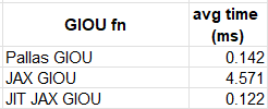
The comparative results appear in the table below:
Avg time of different GIOU implementations (lower is better) — by Author
We can see that JIT-compiling our naive JAX implementation results in slightly better performance than our Pallas kernel. Once again, we can see that matching or surpassing the performance results of JIT compilation (and its inherent kernel fusion) would require fine-tuning of our custom kernel.
Utilizing the Sequential Nature of TPUs
While the ability to develop custom kernels for TPU offers great potential, our examples thus far have demonstrated that reaching optimal runtime performance could be challenging. One way to overcome this is to seek opportunities to utilize the unique properties of the TPU architecture. One example of this is the sequential nature of the TPU processor. Although deep learning workloads tend to rely on operations that are easily parallelizable (e.g., matrix multiplication), on occasion they require algorithms that are inherently sequential. These can pose a serious challenge for the SIMT (single instruction multi thread) model of GPUs and can sometimes have a disproportionate impact on runtime performance. In a sequel to this post, we demonstrate how we can implement sequential algorithms in a way that takes advantage of the TPUs sequential processor and in a manner that minimizes their performance penalty.
Summary
The introduction of Pallas marks an important milestone in the evolution of TPUs. By enabling customization of TPU operations it can potentially unlock new opportunities for TPU programmability, particularly in the world of ML. Our intention in this post was to demonstrate the accessibility of this powerful new feature. While our examples have indeed shown this, they have also highlighted the effort required to reach optimal runtime performance.
We use cookies on our website to give you the most relevant experience by remembering your preferences and repeat visits. By clicking “Accept”, you consent to the use of ALL the cookies.
This website uses cookies to improve your experience while you navigate through the website. Out of these, the cookies that are categorized as necessary are stored on your browser as they are essential for the working of basic functionalities of the website. We also use third-party cookies that help us analyze and understand how you use this website. These cookies will be stored in your browser only with your consent. You also have the option to opt-out of these cookies. But opting out of some of these cookies may affect your browsing experience.
Necessary cookies are absolutely essential for the website to function properly. These cookies ensure basic functionalities and security features of the website, anonymously.
Cookie
Duration
Description
cookielawinfo-checkbox-analytics
11 months
This cookie is set by GDPR Cookie Consent plugin. The cookie is used to store the user consent for the cookies in the category "Analytics".
cookielawinfo-checkbox-functional
11 months
The cookie is set by GDPR cookie consent to record the user consent for the cookies in the category "Functional".
cookielawinfo-checkbox-necessary
11 months
This cookie is set by GDPR Cookie Consent plugin. The cookies is used to store the user consent for the cookies in the category "Necessary".
cookielawinfo-checkbox-others
11 months
This cookie is set by GDPR Cookie Consent plugin. The cookie is used to store the user consent for the cookies in the category "Other.
cookielawinfo-checkbox-performance
11 months
This cookie is set by GDPR Cookie Consent plugin. The cookie is used to store the user consent for the cookies in the category "Performance".
viewed_cookie_policy
11 months
The cookie is set by the GDPR Cookie Consent plugin and is used to store whether or not user has consented to the use of cookies. It does not store any personal data.
Functional cookies help to perform certain functionalities like sharing the content of the website on social media platforms, collect feedbacks, and other third-party features.
Performance cookies are used to understand and analyze the key performance indexes of the website which helps in delivering a better user experience for the visitors.
Analytical cookies are used to understand how visitors interact with the website. These cookies help provide information on metrics the number of visitors, bounce rate, traffic source, etc.
Advertisement cookies are used to provide visitors with relevant ads and marketing campaigns. These cookies track visitors across websites and collect information to provide customized ads.