In this post, we will demonstrate how to set up Slack connector for Amazon Q Business to sync communications from both public and private channels, reflective of user permissions.
In this post, we provide an overview of the alternate AWS services that offer anomaly detection capabilities for customers to consider transitioning their workloads to.
Google Colab and its integrated Generative AI, a powerful combination
Image by author, realized with DALL-E.
What you’ll find in this article: A guide on the various ways to use Generative AI tools integrated into Google Colab (a no-installation, cloud-based platform for coding in Python), making it the easiest way to learn and work with Python.
Knowing how to code is more useful and more accessible than ever. In this article you’ll see how to start coding in a minute without any prerequisites, leveraging the power of the latest Generative AI tools.
I started coding 25 years ago; I was about 10 years old. Everything was tough, from installing development tools, to learning the commands, including debugging of course.
Today, we are very far from that era. Google Colab recently integrated a set of GenAI tools that completely revolutionize the way we code.
It has never been easier to start coding. All the barriers are now down.
This is great news because coding is virtually everywhere and becoming useful, or even required, in a growing number of jobs. Moreover, if you know a little bit of code, you can now go extremely far with minimal effort thanks to these Generative AI tools.
In this article, I will show you the most efficient way to learn and use Python today with a no-installation tool. If you are not new to Python (know what Google Colab and notebooks are, you can skip Part I). The article is organized as follows:
Part I: Preliminary:
Why choose Python and Google Colab?
Where to start learning Python?
Part II: Generative AI tools integrated in Google Colab:
Code completion
Debugging
Suggestions
Graph suggestion
Getting help
Discussion
Part I: Preliminary
Why choose Python and Google Colab?
Why Python? Python is the most popular and versatile language today. Python can be used for:
Machine Learning and Artificial Intelligence (e.g. NLP, deep learning),
Statistics and Analytics
Creating and working with Chatbots (e.g. LLMs, agents etc.)
Web development (e.g. Backend Development)
and more: Finance, Robotics, Database access, Game development etc.
Moreover, due to its popularity, Python is a requirement for many jobs, and it’s particularly easy to learn because of the vast number of resources available.
Why Google Colab? When it comes to Python there are numerous ways to code. The two most popular ways to start are IDEs (Integrated Development Environments) or Notebooks. Notebooks are a web-based interactive environment for writing code. They allow you to mix code, text, and visualizations in a single document.
You can either install a local notebook tool on your computer (e.g. Jupyter Notebook) or use an online cloud-based solution like Google Colab.
Since this guide is focused on accessibility, I picked a cloud-based tool that requires no installation. The only requirement is a Google account. All the documents will be stored on your Google Drive, and hence you can work from any computer and easily collaborate with others.
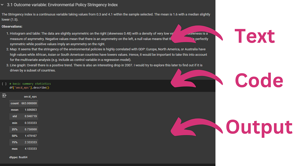
This is a snippet of a Notebook (Google Colab). You can see that in the same document, you have texts, code and the output of the code. Image by author
Where to start learning Python?
There are countless options to start learning Python. Here are two sources for a complete beginner’s guide to Python in different formats:
Learning how to code is similar to learning many other skills, like swimming or biking — you need to practice. So, when you start with these tutorials or others, open Google Colab, start experimenting with code, and adapt it. Use the tools covered in Part II to support your learning journey.
Part II: Generative AI Tools Integrated in Google Colab
Since the public release of ChatGPT 3.5 in November 2022, the number of Generative AI tools to support coding has grown quickly. Large Language Models, like ChatGPT, are incredibly powerful to help us with code. Coding relies on a “language” with clear syntax, which makes it an ideal domain for LLMs.
Google Colab recently integrated a set of Generative AI tools that can support various aspects of your work, from code suggestions to debugging and explanations. Let’s now cover all of these tools:
Code completion
Debugging
Suggestions
Automatic graphs suggestions
Help
Code completion
When you start typing code in Google Colab, you’ll quickly notice that code suggestions appear in grey and italic (see video below) beyond what you type.
The suggestions appear very quickly and adapt as you continue typing. You just need to press the Tab key to accept the suggestion.
Note that the suggestions are based not only on what you are typing but also on the rest of the file, making this feature incredibly powerful and going significantly beyond traditional simple code completion tools. For example, in the video below, the suggestion for importing a file is not generic — it’s the exact code needed to import the file in my active Google Colab document with the correct format.
This video illustrates the code completion tool in Google Colab. You can see me type the beginning of some line of code in white and then the suggestions automatically and very quickly appear in grey and italic. I just have to click the Tab key to accept the suggestion. Video by author.
Debugging
If you’ve ever tried coding, you know that debugging is often what we spend the most time doing. Historically, if you didn’t understand the error, you would refer to manuals, copy and paste the error message, and search online (e.g. Stack Overflow) for solutions. More recently, you might even ask ChatGPT or another LLM for help.
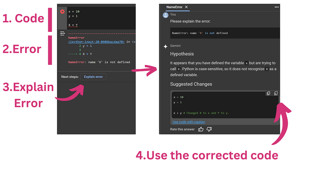
But now there’s an incredibly fast integrated solution. As you can see in the video below, I ran some code that generated an error. After each error message, you’ll see a button labeled “Explain error.” Once you click it, a pane will open on the right-hand side, and Gemini (an LLM) will explain the error and propose adjusted code. You can then adapt the code by hand, copy-paste the suggestion, or in one click, create a new cell with the corrected code in your notebook.
Here is an example of a simple debugging situation with the integrated Generative AI system in Google Colab. Image by author.
Suggestions
Beyond code completion, Google Colab offers two simple ways to suggest code based on your description.
The first way is by writing a comment (see the video below). I just write a comment that explains the next line of code, and Colab directly interprets it and automatically suggests the corresponding code. This functionality works mainly for simple, usually single lines of code.
This video illustrate how Google Colab use Generative AI to automatically generate the code corresponding the the comment you just wrote. Video by author.
When you need code suggestions for more complex requests, often requiring several lines of code, you can click on “Generate” with AI when you start a new code block (see video below). Then, you can use natural language to explain what you want to do, and the code will be automatically generated. Note that the prompt will be included as a comment on top, so try to make a clear request to save time.
This video illustrate how you can use natural language to create code in Google Colab. Video by author.
Automatic graphs suggestions
There are also specific suggestions for graph creation when you work with a dataframe (see video below). When you describe or display part of a dataframe, an icon with a graph appears in the top right corner. When you click on it, you’ll see a gallery of potential graphs. By clicking on one of the graphs, a new code cell will be generated with the code required to create the selected graph.
So far, I haven’t been very impressed by this function. It crashed a few times, returned errors, or suggested numerous options, but the one I was interested in wasn’t available.
This video illustrates the automatic graph suggestion in Google Copilot. Video by author.
Help
Finally, you can directly chat with Gemini (a chatbot/LLM) to ask code-related questions. These questions could be about a piece of code you don’t understand, how to perform a specific task with code, or virtually anything else. You essentially have an AI tutor available 24/7, just one click away.
You can click on the top right button “Gemini” in Google Colab to directly start a discussion about code. You can ask questions about current code, about how to do something etc. Image by author.
Discussion
While Generative AI is incredibly useful and powerful for coding, it should be used in moderation when learning. This efficiency might prevent us from truly mastering the material and could negatively affect our long-term performance.
I was blown away by the impact of these Generative AI integrations. I find myself writing less and less code — it’s more about being able to read and test code now. But reading is always easier than writing, just like when learning any language (not just programming).
However, this raises questions about the long-term effects for people who haven’t yet fully learned how to code. I remember using these tools extensively to select parts of Pandas dataframes because I often mixed up the brackets, .loc or .iloc functions, and syntax. ChatGPT helped me go faster a few times, but over the long run, I became less efficient. If I have to ask every time, it often takes longer than if I knew the solution by heart. And what happens if the tool isn’t available?
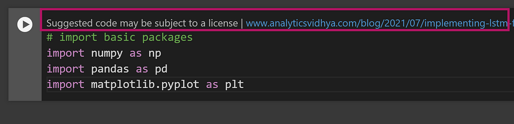
Moreover, it’s very important to remember to use AI suggestions responsibly. Always aim to understand the code you’re incorporating to avoid potential issues with plagiarism or unintended errors. Note that when using suggestions in Google Colab, you might see the source of the code inspiration (see image below). This information can help you avoid potential copyright violations.
Example of a note added in Google Colab when using a Generative AI code recommendation. It appears that the potential source of the code is cited, and a clickable link is available to check for any potential copyright issues. Image by author.
A/B Testing, Reject Inference, and How to Get the Right Sample Size for Your Experiments
Image created by the author
There are different statistical formulas for different scenarios. The first question to ask is: are you comparing two groups, such as in an A/B test, or are you selecting a sample from a population that is large enough to represent it?
The latter is typically used in cases like holdout groups in transactions. These holdout groups can be crucial for assessing the performance of fraud prevention rules or for reject inference, where machine learning models for fraud detection are retrained. The holdout group is beneficial because it contains transactions that weren’t blocked by any rules or models, providing an unbiased view of performance. However, to ensure the holdout group is representative, you need to select a sample size that accurately reflects the population, which, together with sample sizing for A/B testing, we’ll explore it in this article.
After determining whether you’re comparing two groups (like in A/B testing) or taking a representative sample (like for reject inference), the next step is to define your success metric. Is it a proportion or an absolute number? For example, comparing two proportions could involve conversion rates or default rates, where the number of default transactions is divided by the total number of transactions. On the other hand, comparing two means applies when dealing with absolute values, such as total revenue or GMV (Gross Merchandise Value). In this case, you would compare the average revenue per customer, assuming customer-level randomization in your experiment.
1. Comparing two groups (e.g. A/B testing) — Sample Size
The section 1.1 is about comparing two means, but most of the principles presented there will be the same for section 1.2.
1.1. Comparing two Means (metric the average of an absolute number)
In this scenario, we are comparing two groups: a control group and a treatment group. The control group consists of customers with access to €100 credit through a lending program, while the treatment group consists of customers with access to €200 credit under the same program.
The goal of the experiment is to determine whether increasing the credit limit leads to higher customer spending.
Our success metric is defined as the average amount spent per customer per week, measured in euros.
With the goal and success metric established, in a typical A/B test, we would also define the hypothesis, the randomization unit (in this case, the customer), and the target population (new customers granted credit). However, since the focus of this document is on sample size, we will not go into those details here.
We will compare the average weekly spending per customer between the control group and the treatment group. Let’s proceed with calculating this metric using the following script:
Script 1: Computing the success metric, branch: Germany, period: 2024–05–01 to 2024–07–31.
WITH customer_spending AS (
SELECT
 branch_id,
 FORMAT_DATE('%G-%V', DATE(transaction_timestamp)) AS week_of_year,
 customer_id,
 SUM(transaction_value) AS total_amount_spent_eur
FROM `project.dataset.credit_transactions`
WHERE 1=1
 AND transaction_date BETWEEN '2024-05-01' AND '2024-07-31'
 AND branch_id LIKE 'Germany'
GROUP BY branch_id, week_of_year, customer_id
)
, agg_per_week AS (
SELECT
 branch_id,
 week_of_year,
 ROUND(AVG(total_amount_spent_eur), 1) AS avg_amount_spent_eur_per_customer,
FROM customer_spending
GROUP BY branch_id, week_of_year
)
SELECT *
FROM agg_per_week
ORDER BY 1,2;
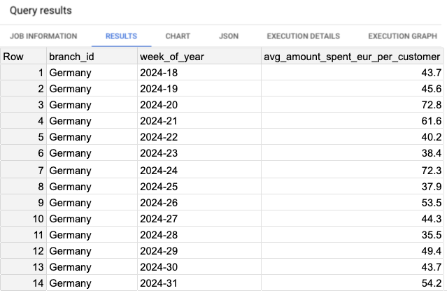
In the results, we observe the metric avg_amount_spent_eur_per_customer on a weekly basis. Over the last four weeks, the values have remained relatively stable, ranging between 35 and 54 euros. However, when considering all weeks over the past two months, the variance is higher. (See Image 1 for reference.)
Image 1: Results of the script 1.
Next, we calculate the variance of the success metric. To do this, we will use Script 2 to compute both the variance and the average of the weekly spending across all weeks.
Script 2: Query to compute the variance of the success metric and average over all weeks.
WITH customer_spending AS (
SELECT
 branch_id,
 FORMAT_DATE('%G-%V', DATE(transaction_timestamp)) AS week_of_year,
 customer_id,
 SUM(transaction_value) AS total_amount_spent_eur
FROM `project.dataset.credit_transactions`
WHERE 1=1
 AND transaction_date BETWEEN '2024-05-01' AND '2024-07-31'
 AND branch_id LIKE 'Germany'
GROUP BY branch_id, week_of_year, customer_id
)
, agg_per_week AS (
SELECT
 branch_id,
 week_of_year,
 ROUND(AVG(total_amount_spent_eur), 1) AS avg_amount_spent_eur_per_customer,
FROM customer_spending
GROUP BY branch_id, week_of_year
)
SELECT
 ROUND(AVG(avg_amount_spent_eur_per_customer),1) AS avg_amount_spent_eur_per_customer_per_week,
 ROUND(VAR_POP(avg_amount_spent_eur_per_customer),1) AS variance_avg_amount_spent_eur_per_customer
FROM agg_per_week
ORDER BY 1,2;
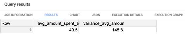
The result from Script 2 shows that the variance is approximately 145.8 (see Image 2). Additionally, the average amount spent per user, considering all weeks over the past two months, is 49.5 euros.
Image 2: Results of Script 2.
Now that we’ve calculated the metric and found the average weekly spending per customer to be approximately 49.5 euros, we can define the Minimum Detectable Effect (MDE). Given the increase in credit from €100 to €200, we aim to detect a 10% increase in spending, which corresponds to a new average of 54.5 euros per customer per week.
With the variance calculated (145.8) and the MDE established, we can now plug these values into the formula to calculate the sample size required. We’ll use default values for alpha (5%) and beta (20%):
Significance Level (Alpha’s default value is α = 5%): The alpha is a predetermined threshold used as a criteria to reject the null hypothesis. Alpha is the type I error (false positive), and the p-value needs to be lower than the alpha, so that we can reject the null hypothesis.
Statistical Power (Beta’s default value is β = 20%): It’s the probability that a test correctly rejects the null hypothesis when the alternative hypothesis is true, i.e. detecting an effect when the effect is present. Statistical Power = 1 — β, and β is the type II error (false negative).
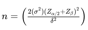
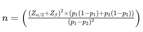
Here is the formula to calculate the required sample size per group (control and treatment) for comparing two means in a typical A/B test scenario:
Image 3: Formula to calculate sample size when comparing two means.
n is the sample size per group.
σ² is the variance of the metric being tested (in this case, 145.8). The factor 2σ² is used because we calculate the pooled variance, making it unbiased when comparing two samples.
δ (Delta), represents the minimum detectable difference in means (effect size), which is the change we want to detect. That is calculated as: δ² = (μ₁ — μ₂)² , where μ₁ is the mean of the control group and μ₂ is the mean of the treatment group.
Zα/2 is the z-score for the corresponding confidence level (e.g., 1.96 for 95% confidence level).
Zβ is the z-score associated with the desired power of the test (e.g., 0.84 for 80% power).
n = (2 * 145.8 * (1.96+0.84)^2) / (54.5-49.5)^2
-> n = 291.6 * 7.84 / 25
-> n = 2286.1 / 25
-> n =~ 92
Try it on my web app calculator at Sample Size Calculator, as shown in App Screenshot 1:
Confidence Level: 95%
Statistical Power: 80%
Variance: 145.8
Difference to Detect (Delta): 5 (because the expected change is from €49.50 to €54.50)
App screenshot 1: Calculating the sample for comparing two means.
Based on the previous calculation, we would need 92 users in the control group and 92 users in the treatment group, for a total of 184 samples.
Now, let’s explore how changing the Minimum Detectable Effect (MDE) impacts the sample size. Smaller MDEs require larger sample sizes. For example, if we were aiming to detect a change of only €1 increase on average per user, instead of the €5 increase (10%) we used previously, the required sample size would increase significantly.
The smaller the MDE, the more sensitive the test needs to be, which means we need a larger sample to reliably detect such a small effect.
n = (2 * 145.8 * (1.96+0.84)^2) / (50.5-49.5)^2
-> n = 291.6 * 7.84 / 1
-> n = 2286.1 / 1
-> n =~ 2287
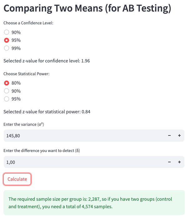
We enter the following parameters into the web app calculator at Sample Size Calculator, as shown in App Screenshot 2:
Confidence Level: 95%
Statistical Power: 80%
Variance: 145.8
Difference to Detect (Delta): 1 (because the expected change is from €49.50 to €50.50)
App screenshot 2: Calculating the sample for comparing two means with Delta = 1.
To detect a smaller effect, such as a €1 increase per user, we would require 2,287 users in the control group and 2,287 users in the treatment group, resulting in a total of 4,574 samples.
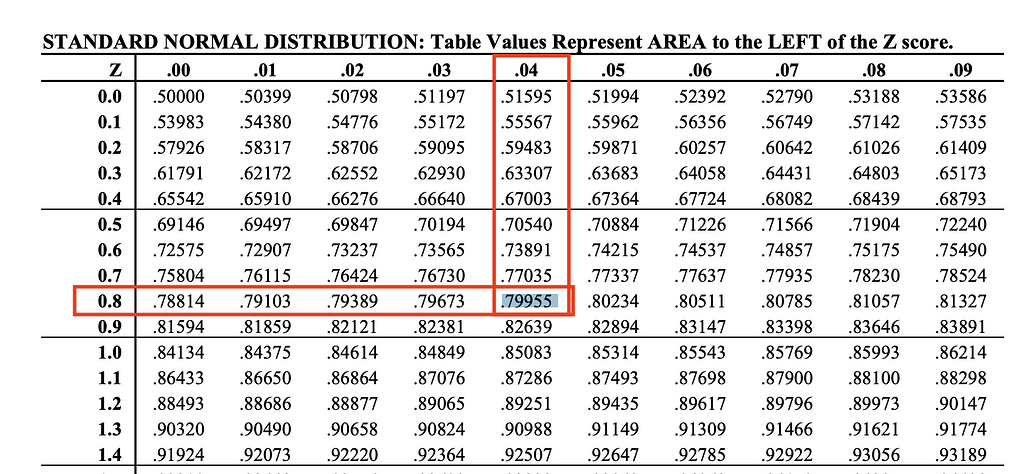
Next, we’ll adjust the statistical power and significance level to recompute the required sample size. But first, let’s take a look at the z-score table to understand how the Z-value is derived.
We’ve set beta = 0.2, meaning the current statistical power is 80%. Referring to the z-score table (see Image 4), this corresponds to a z-score of 0.84, which is the value used in our previous formula.
Image 4: Finding the z-score for a statistical power of 80% on z-score table.
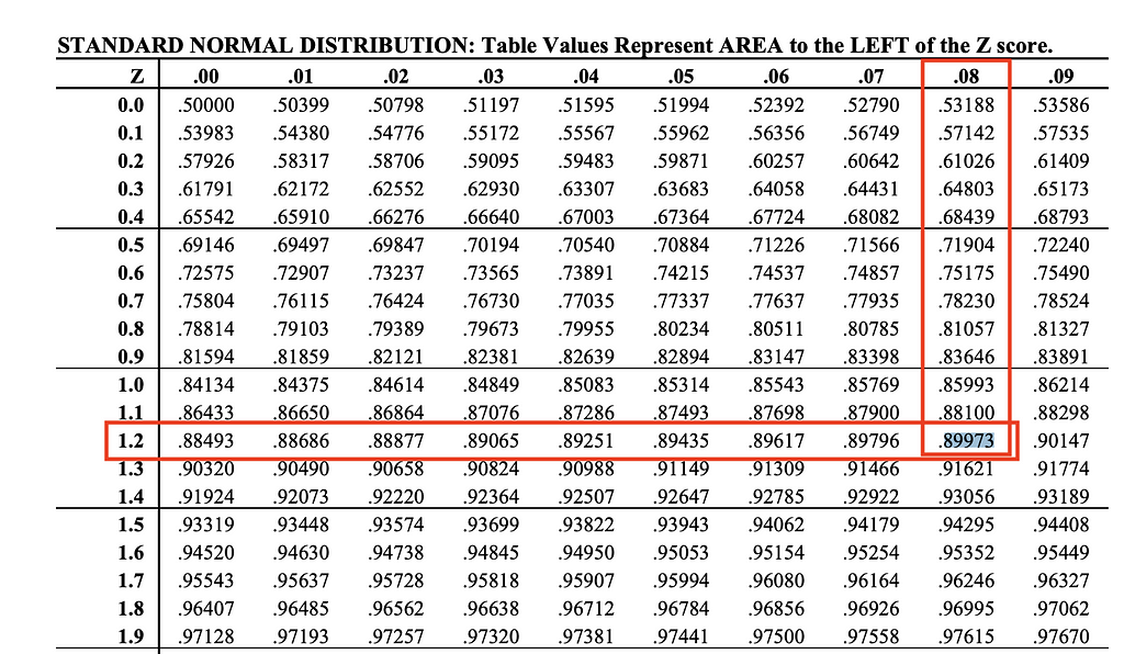
If we now adjust beta to 10%, which corresponds to a statistical power of 90%, we will find a z-value of 1.28. This value can be found on the z-score table (see Image 5).
n = (2 * 145.8 * (1.96+1.28)^2) / (50.5-49.5)^2
-> n = 291.6 * 10.49 / 1
-> n = 3061.1 / 1
-> n =~ 3062
With the adjustment to a beta of 10% (statistical power of 90%) and using the z-value of 1.28, we now require 3,062 users in both the control and treatment groups, for a total of 6,124 samples.
Image 5: Finding the z-score for a statistical power of 90% on the z-score table.
Now, let’s determine how much traffic the 6,124 samples represent. We can calculate this by finding the average volume of distinct customers per week. Script 3 will help us retrieve this information using the time period from 2024–05–01 to 2024–07–31.
Script 3: Query to calculate the average weekly volume of distinct customers.
WITH customer_volume AS (
SELECT
 branch_id,
 FORMAT_DATE('%G-%V', DATE(transaction_timestamp)) AS week_of_year,
 COUNT(DISTINCT customer_id) AS cntd_customers
FROM `project.dataset.credit_transactions`
WHERE 1=1
 AND transaction_date BETWEEN '2024-05-01' AND '2024-07-31'
 AND branch_id LIKE 'Germany'
GROUP BY branch_id, week_of_year
)
SELECT
 ROUND(AVG(cntd_customers),1) AS avg_cntd_customers
FROM customer_volume;
The result from Script 3 shows that, on average, there are 185,443 distinct customers every week (see Image 5). Therefore, the 6,124 samples represent approximately 3.35% of the total weekly customer base.
Image 5: Results from Script 3.
1.2. Comparing two Proportions (e.g. conversion rate, default rate)
While most of the principles discussed in the previous section remain the same, the formula for comparing two proportions differs. This is because, instead of pre-computing the variance of the metric, we will now focus on the expected proportions of success in each group (see Image 6).
Image 6: Formula to calculate sample size for comparing two proportions.
Let’s return to the same scenario: we are comparing two groups. The control group consists of customers who have access to €100 credit on the credit lending program, while the treatment group consists of customers who have access to €200 credit in the same program.
This time, the success metric we are focusing on is the default rate. This could be part of the same experiment discussed in Section 1.1, where the default rate acts as a guardrail metric, or it could be an entirely separate experiment. In either case, the hypothesis is that giving customers more credit could lead to a higher default rate.
The goal of this experiment is to determine whether an increase in credit limits results in a higher default rate.
We define the success metric as the average default rate for all customers during the experiment week. Ideally, the experiment would run over a longer period to capture more data, but if that’s not possible, it’s essential to choose a week that is unbiased. You can verify this by analyzing the default rate over the past 12–16 weeks to identify any specific patterns related to certain weeks of the month.
Let’s examine the data. Script 4 will display the default rate per week, and the results can be seen in Image 7.
Script 4: Query to retrieve default rate per week.
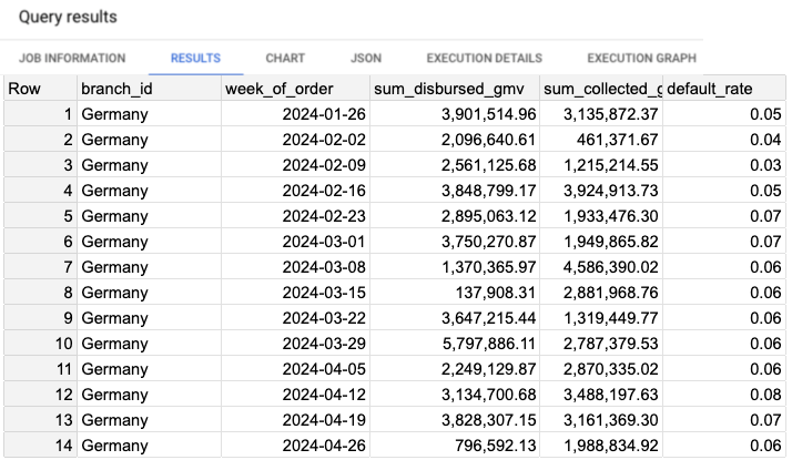
SELECT
 branch_id,
 date_trunc(transaction_date, week) AS week_of_order,
 SUM(transaction_value) AS sum_disbursed_gmv,
 SUM(CASE WHEN is_completed THEN transaction_value ELSE 0 END) AS sum_collected_gmv,
 1-(SUM(CASE WHEN is_completed THEN transaction_value ELSE 0 END)/SUM(transaction_value)) AS default_rate,
FROM `project.dataset.credit_transactions`
WHERE transaction_date BETWEEN '2024-02-01' AND '2024-04-30'
  AND branch_id = 'Germany'
GROUP BY 1,2
ORDER BY 1,2;
Looking at the default rate metric, we notice some variability, particularly in the older weeks, but it has remained relatively stable over the past 5 weeks. The average default rate for the last 5 weeks is 0.070.
Image 7: Results of the default rate per week.
Now, let’s assume that this default rate will be representative of the control group. The next question is: what default rate in the treatment group would be considered unacceptable? We can set the threshold: if the default rate in the treatment group increases to 0.075, it would be too high. However, anything up to 0.0749 would still be acceptable.
A default rate of 0.075 represents approximately 7.2% increase from the control group rate of 0.070. This difference — 7.2% — is our Minimum Detectable Effect (MDE).
With these data points, we are now ready to compute the required sample size.
n = ( ((1.96+0.84)^2) * ((0.070*(1-0.070) + 0.075*(1-0.075)) ) / ( (0.070-0.075)^2 )
-> n = 7.84 * 0.134475 / 0.000025
-> n = 1.054284 / 0.000025
-> n =~ 42,171
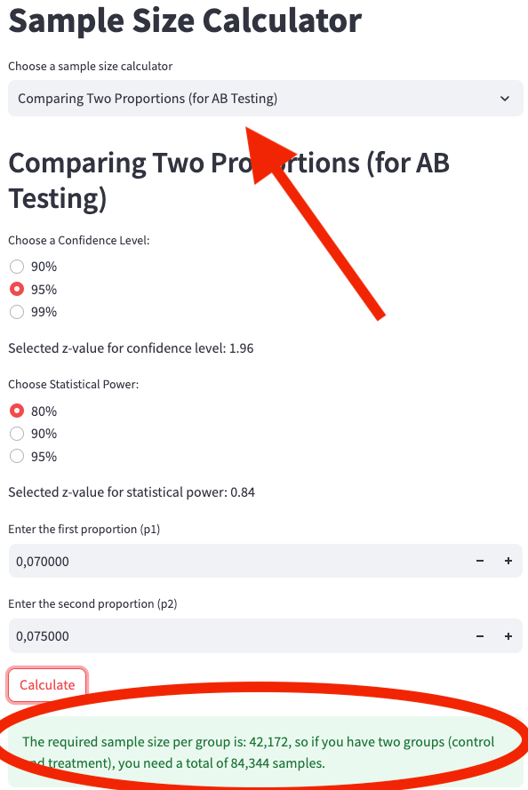
We enter the following parameters into the web app calculator at Sample Size Calculator, as shown in App Screenshot 3:
Confidence Level: 95%
Statistical Power: 80%
First Proportion (p1): 0.070
Second Proportion (p2): 0.075
App screenshot 3: Calculating the sample size for comparing two proportions.
To detect a 7.2% increase in the default rate (from 0.070 to 0.075), we would need 42,171 users in both the control group and the treatment group, resulting in a total of 84,343 samples.
A sample size of 84,343 is quite large! We may not even have enough customers to run this analysis. But let’s explore why this is the case. We haven’t changed the default parameters for alpha and beta, meaning we kept the significance level at the default 5% and the statistical power at the default 80%. As we’ve discussed earlier, we could have been more conservative by choosing a lower significance level to reduce the chance of false positives, or we could have increased the statistical power to minimize the risk of false negatives.
So, what contributed to the large sample size? Is it the MDE of 7.2%? The short answer: not exactly.
Consider this alternative scenario: we maintain the same significance level (5%), statistical power (80%), and MDE (7.2%), but imagine that the default rate (p₁) was 0.23 (23%) instead of 0.070 (7.0%). With a 7.2% MDE, the new default rate for the treatment group (p₂) would be 0.2466 (24.66%). Notice that this is still a 7.2% MDE, but the proportions are significantly higher than 0.070 (7.0%) and 0.075 (7.5%).
Now, when we perform the sample size calculation using these new values of p₁ = 0.23 and p₂ = 0.2466, the results will differ. Let’s compute that next.
n = ( ((1.96+0.84)^2) * ((0.23*(1-0.23) + 0.2466*(1-0.2466)) ) / ( (0.2466-0.23)^2 )
-> n = 7.84 * 0.3628 / 0.00027556
-> n = 2.8450 / 0.00027556
-> n =~ 10,325
With the new default rates (p₁ = 0.23 and p₂ = 0.2466), we would need 10,325 users in both the control and treatment groups, resulting in a total of 20,649 samples. This is much more manageable compared to the previous sample size of 84,343. However, it’s important to note that the default rates in this scenario are in a completely different range.
The key takeaway is that lower success rates (like default rates around 7%) require larger sample sizes. When the proportions are smaller, detecting even modest differences (like a 7.2% increase) becomes more challenging, thus requiring more data to achieve the same statistical power and significance level.
2. Sampling a population
This case differs from the A/B testing scenario, as we are now focusing on determining a sample size from a single group. The goal is to take a sample that accurately represents the population, allowing us to run an analysis and then extrapolate the results to estimate what would happen across the entire population.
Even though we are not comparing two groups, sampling from a population (a single group) still requires deciding whether you are estimating a mean or a proportion. The formulas for these scenarios are quite similar to those used in A/B testing.
Take a look at images 8 and 9. Did you notice the similarities when comparing image 8 with image 3 (sample size formula for comparing two means) and when comparing image 9 with image 6 (sample size formula for comparing two proportions)? They are indeed quite similar.
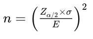
Image 8: Sample size formula to estimate the mean of a population.
In the case of estimating the mean:
From image 8, the formula for sampling from one group, however, uses E, which stands for the Error.
From image 3, the formula for comparing two groups uses delta (δ) to compare the difference between the two means.
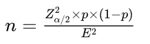
Image 9: Sample size formula to estimate the proportion of a population.
In the case of estimating proportions:
From image 9, for sampling from a single group, the formula for proportions also uses E instead, representing the Error.
From image 6, the formula for comparing two groups uses the MDE (Minimum Detectable Effect), similar to delta, to compare the difference between two proportions.
Now, when should we use each of these formulas? Let’s explore two practical examples — one for estimating a mean and another for estimating a proportion.
2.1. Sampling a population — Estimating the mean
Let’s say you want to better assess the risk of fraud, and to do so, you aim to estimate the average order value of fraudulent transactions by country and per week. This can be quite challenging because, ideally, most fraudulent transactions are already being blocked. To get a clearer picture, you would take a holdout group that is free of rules and models, which would serve as a reference for calculating the true average order value of fraudulent transactions.
Suppose you select a specific country, and after reviewing historical data, you find that:
The variance of this metric is €905.
The average order value of fraudulent transactions is €100. (You can refer to Scripts 1 and 2 for calculating the success metric and variance.)
Since the variance is €905, the standard deviation (square root of variance) is approximately €30. Now, using a significance level of 5%, which corresponds to a z-score of 1.96, and assuming you’re comfortable with a 10% margin of error (representing an Error of €10, or 10% of €100), the confidence interval at 95% would mean that with the correct sample size, you can say with 95% confidence that the average value falls between €90 and €110.
Now, plugging these inputs into the sample size formula:
n = ( (1.96 * 30) / 10 )^2
-> n = (58.8/10)^2
-> n = 35
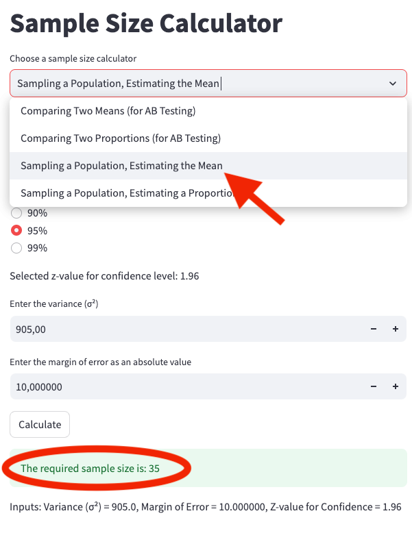
We enter the following parameters into the web app calculator at Sample Size Calculator, as shown in App Screenshot 4:
Confidence Level: 95%
Variance: 905
Error: 10
App screenshot 4: Calculating the sample size for estimating the mean when sampling a population.
The result is that you would need 35 samples to estimate the average order value of fraudulent transactions per country per week. However, that’s not the final sample size.
Since fraudulent transactions are relatively rare, you need to adjust for the proportion of fraudulent transactions. If the proportion of fraudulent transactions is 1%, the actual number of samples you need to collect is:
n = 35/0.01
-> n = 3500
Thus, you would need 3,500 samples to ensure that fraudulent transactions are properly represented.
2.2. Sampling a population — Estimating a proportion
In this scenario, our fraud rules and models are blocking a significant number of transactions. To assess how well our rules and models perform, we need to let a portion of the traffic bypass the rules and models so that we can evaluate the actual false positive rate. This group of transactions that passes through without any filtering is known as a holdout group. This is a common practice in fraud data science teams because it allows for both evaluating rule and model performance and reusing the holdout group for reject inference.
Although we won’t go into detail about reject inference here, it’s worth briefly summarizing. Reject inference involves using the holdout group of unblocked transactions to learn patterns that help improve transaction blocking decisions. Several methods exist for this, with fuzzy augmentation being a popular one. The idea is to relabel previously rejected transactions using the holdout group’s data to train new models. This is particularly important in fraud modeling, where fraud rates are typically low (often less than 1%, and sometimes as low as 0.1% or lower). Increasing labeled data can improve model performance significantly.
Now that we understand the need to estimate a proportion, let’s dive into a practical use case to find out how many samples are needed.
For a certain branch, you analyze historical data and find that it processes 50,000,000 orders in a month, of which 50,000 are fraudulent, resulting in a 0.1% fraud rate. Using a significance level of 5% (alpha) and a margin of error of 25%, we aim to estimate the true fraud proportion within a confidence interval of 95%. This means if the true fraud rate is 0.001 (0.1%), we would be estimating a range between 0.00075 and 0.00125, with an Error of 0.00025.
Please note that margin of error and Error are two different things, the margin of error is a percentage value, and the Error is an absolute value. In the case where the fraud rate is 0.1% if we have a margin of error of 25% that represents an Error of 0.00025.
Let’s apply the formula:
Zα/2 = 1.96 (z-score for 95% confidence level)
E = 0.00025 (Error)
p = 0.001 (fraud rate)
Zalpha/2= 1.96
-> (Zalpha/2)^2= 3.8416
E = 0.00025
-> E^2 = 0.0000000625
p = 0.001

n =( 3.8416 * 0.001 * (1 - 0.001) ) / 0.0000000625
-> n = 0.0038377584 / 0.0000000625
-> n = 61,404
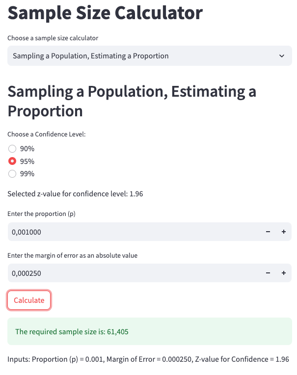
We enter the following parameters into the web app calculator at Sample Size Calculator, as shown in App Screenshot 5:
Confidence Level: 95%
Proportion: 0.001
Error: 0.00025
App screenshot 5: Calculating the sample size for estimating a proportion when sampling a population.
Thus, 61,404 samples are required in total. Given that there are 50,000,000 transactions in a month, it would take less than 1 hour to collect this many samples if the holdout group represented 100% of the traffic. However, this isn’t practical for a reliable experiment.
Instead, you would want to distribute the traffic across several days to avoid seasonality issues. Ideally, you would collect data over at least a week, ensuring representation from all weekdays while avoiding holidays or peak seasons. If you need to gather 61,404 samples in a week, you would aim for 8,772 samples per day. Since the daily traffic is around 1,666,666 orders, the holdout group would need to represent 0.53% of the total transactions each day, running over the course of a week.
Final notes
If you’d like to perform these calculations in Python, here are the relevant functions:
These functions are also available in the GitHub repository: GitHub Sample Size Calculator, this is also where you can find the link to the Interactive Sample Size Calculator.
Disclaimer: The images that resemble the results of a Google BigQuery job have been created by the author. The numbers shown are not based on any business data but were manually generated for illustrative purposes. The same applies to the SQL scripts — they are not from any businesses and were also manually generated. However, they are designed to closely resemble what a company using Google BigQuery as a framework might encounter.
Calculator written in Python and deployed in Google Cloud Run (Serverless environment) using a Docker container and Streamlit, see code in GitHub for reference.
This is a direct sequel to a previous post on the topic of implementing custom TPU operations with Pallas. Of particular interest are custom kernels that leverage the unique properties of the TPU architecture in a manner that optimizes runtime performance. In this post, we will attempt to demonstrate this opportunity by applying the power of Pallas to the challenge of running sequential algorithms that are interspersed within a predominantly parallelizable deep learning (DL) workload.
We will focus on Non Maximum Suppression (NMS) of bounding-box proposals as a representative algorithm, and explore ways to optimize its implementation. An important component of computer vision (CV) object detection solutions (e.g., Mask RCNN), NMS is commonly used to filter out overlapping bounding boxes, keeping only the “best” ones. NMS receives a list of bounding box proposals, an associated list of scores, and an IOU threshold, and proceeds to greedily and iteratively choose the remaining box with the highest score and disqualify all other boxes with which it has an IOU that exceeds the given threshold. The fact that the box chosen at the n-th iteration depends on the preceding n-1 steps of the algorithm dictates the sequential nature of its implementation. Please see here and/or here for more on the rational behind NMS and its implementation. Although we have chosen to focus on one specific algorithm, most of our discussion should carry over to other sequential algorithms.
Offloading Sequential Algorithms to CPU
The presence of a sequential algorithm within a predominantly parallelizable ML model (e.g., Mask R-CNN) presents an interesting challenge. While GPUs, commonly used for such workloads, excel at executing parallel operations like matrix multiplication, they can significantly underperform compared to CPUs when handling sequential algorithms. This often leads to computation graphs that include crossovers between the GPU and CPU, where the GPU handles the parallel operations and the CPU handles the sequential ones. NMS is a prime example of a sequential algorithm that is commonly offloaded onto the CPU. In fact, a close analysis of torchvision’s “CUDA” implementation of NMS, reveals that even it runs a significant portion of the algorithm on CPU.
Although offloading sequential operations to the CPU may lead to improved runtime performance, there are several potential drawbacks to consider:
Cross-device execution between the CPU and GPU usually requires multiple points of synchronization between the devices which commonly results in idle time on the GPU while it waits for the CPU to complete its tasks. Given that the GPU is typically the most expensive component of the training platform our goal is to minimize such idle time.
In standard ML workflows, the CPU is responsible for preparing and feeding data to the model, which resides on the GPU. If the data input pipeline involves compute-intensive processing, this can strain the CPU, leading to “input starvation” on the GPU. In such scenarios, offloading portions of the model’s computation to the CPU could further exacerbate this issue.
To avoid these drawbacks you could consider alternative approaches, such as replacing the sequential algorithm with a comparable alternative (e.g., the one suggested here), settling for a slow/suboptimal GPU implementation of the sequential algorithm, or running the workload on CPU — each of which come with there own potential trade-offs.
Sequential Algorithms on TPU
This is where the unique architecture of the TPU could present an opportunity. Contrary to GPUs, TPUs are sequential processors. While their ability to run highly vectorized operations makes them competitive with GPUs when running parallelizable operations such as matrix multiplication, their sequential nature could make them uniquely suited for running ML workloads that include a mix of both sequential and parallel components. Armed with the Pallas extension to JAX, our newfound TPU kernel creation tool, we will evaluate this opportunity by implementing and evaluating a custom implementation of NMS for TPU.
Disclaimers
The NMS implementations we will share below are intended for demonstrative purposes only. We have not made any significant effort to optimize them or to verify their robustness, durability, or accuracy. Please keep in mind that, as of the time of this writing, Pallas is an experimental feature — still under active development. The code we share (based on JAX version 0.4.32) may become outdated by the time you read this. Be sure to refer to the most up-to-date APIs and resources available for your Pallas development. Please do not view our mention of any algorithm, library, or API as an endorsement for their use.
NMS on CPU
We begin with a simple implementation of NMS in numpy that will serve as a baseline for performance comparison:
To evaluate the performance of our NMS function, we generate a batch of random boxes and scores (as JAX tensors) and run the script on a Google Cloud TPU v5e system using the same environment and same benchmarking utility as in our previous post. For this experiment, we specify the CPU as the JAX default device:
import jax from jax import random import jax.numpy as jnp
time = benchmark(nms_cpu)(rand_boxes, rand_scores, max_output_size=128) print(f'nms_cpu: {time}')
The resultant average runtime is 2.99 milliseconds. Note the assumption that the input and output tensors reside on the CPU. If they are on the TPU, then the time to copy them between the devices should also be taken into consideration.
NMS on TPU
If our NMS function is a component within a larger computation graph running on the TPU, we might prefer a TPU-compatible implementation to avoid the drawbacks of cross-device execution. The code block below contains a JAX implementation of NMS specifically designed to enable acceleration via JIT compilation. Denoting the number of boxes by N, we begin by calculating the IOU between each of the N(N-1) pairs of boxes and preparing an NxN boolean tensor (mask_threshold)where the (i,j)-th entry indicates whether the IOU between boxes i and j exceed the predefined threshold.
To simplify the iterative selection of boxes, we create a copy of the mask tensor (mask_threshold2) where the diagonal elements are zeroed to prevent a box from suppressing itself. We further define two score-tracking tensors: out_scores, which retains the scores of the chosen boxes (and zeros the scores of the eliminated ones), and remaining_scores, which maintains the scores of the boxes still being considered. We then use the jax.lax.while_loop function to iteratively choose boxes while updating the out_scores and remaining_scores tensors. Note that the format of the output of this function differs from the previous function and may need to be adjusted to fit into subsequent steps of the computation graph.
import functools
# Given N boxes, calculates mask_threshold an NxN boolean mask # where the (i,j) entry indicates whether the IOU of boxes i and j # exceed the threshold. Returns mask_threshold, mask_threshold2 # which is equivalent to mask_threshold with zero diagonal and # the scores modified so that all values are greater than 0 def init_tensors(boxes, scores, threshold=0.1): epsilon = 1e-5
# Extract left, top, right, bottom coordinates left = boxes[:, 0] top = boxes[:, 1] right = boxes[:, 2] bottom = boxes[:, 3]
# Compute areas of boxes areas = (right - left) * (bottom - top)
# The out_scores tensor will retain the scores of the chosen boxes # and zero the scores of the eliminated ones # remaining_scores will maintain non-zero scores for boxes that # have not been chosen or eliminated remaining_scores = out_scores.copy()
def choose_box(state): i, remaining_scores, out_scores = state # choose index of box with highest score from remaining scores index = jnp.argmax(remaining_scores) # check validity of chosen box valid = remaining_scores[index] > 0 # If valid, zero all scores with IOU greater than threshold # (including the chosen index) remaining_scores = jnp.where(mask_threshold[index] *valid, 0, remaining_scores) # zero the scores of the eliminated tensors (not including # the chosen index) out_scores = jnp.where(mask_threshold2[index]*valid, 0, out_scores)
i = i + 1 return i, remaining_scores, out_scores
def cond_fun(state): i, _, _ = state return (i < max_output_size)
# Output the resultant scores. To extract the chosen boxes, # Take the max_output_size highest scores: # min = jnp.minimum(jnp.count_nonzero(scores), max_output_size) # indexes = jnp.argsort(out_scores, descending=True)[:min] return out_scores
# nms_jax can be run on either the CPU the TPU rand_boxes, rand_scores = generate_random_boxes(run_on_cpu=True)
time = benchmark(nms_jax)(rand_boxes, rand_scores, max_output_size=128) print(f'nms_jax on CPU: {time}')
time = benchmark(nms_jax)(rand_boxes, rand_scores, max_output_size=128) print(f'nms_jax on TPU: {time}')
The runtimes of this implementation of NMS are 1.231 and 0.416 milliseconds on CPU and TPU, respectively.
Custom NMS Pallas Kernel
We now present a custom implementation of NMS in which we explicitly leverage the fact that on TPUs Pallas kernels are executed in a sequential manner. Our implementation uses two boolean matrix masks and two score-keeping tensors, similar to the approach in our previous function.
We define a kernel function, choose_box, responsible for selecting the next box and updating the score-keeping tensors, which are maintained in scratch memory. We invoke the kernel across a one-dimensional grid where the number of steps (i.e., the grid-size) is determined by the max_output_size parameter.
Note that due to some limitations (as of the time of this writing) on the operations supported by Pallas, some acrobatics are required to implement both the “argmax” function and the validity check for the selected boxes. For the sake of brevity, we omit the technical details and refer the interested reader to the comments in the code below.
from jax.experimental import pallas as pl from jax.experimental.pallas import tpu as pltpu
# argmax helper function def pallas_argmax(scores, n_boxes): # we assume that the index of each box is stored in the # least significant bits of the score (see below) idx = jnp.max(scores.astype(float)).astype(int) % n_boxes return idx
# In order to work around the Pallas argsort limitation # we create a new scores tensor with the same ordering of # the input scores tensor in which the index of each score # in the ordering is encoded in the least significant bits sorted = jnp.argsort(scores, descending=True)
time = benchmark(nms_pallas)(rand_boxes, rand_scores, max_output_size=128) print(f'nms_pallas: {time}')
The average runtime of our custom NMS operator is 0.139 milliseconds, making it roughly three times faster than our JAX-native implementation. This result highlights the potential of tailoring the implementation of sequential algorithms to the unique properties of the TPU architecture.
Note that in our Pallas kernel implementation, we load the full input tensors into TPU VMEM memory. Given the limited the capacity of VMEM, scaling up the input size (i.e., increase the number of bounding boxes) will likely lead to memory issues. Typically, such limitations can be addressed by chunking the inputs with BlockSpecs. Unfortunately, applying this approach would break the current NMS implementation. Implementing NMS across input chunks would require a different design, which is beyond the scope of this post.
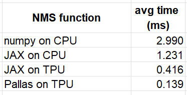
Results
The results of our experiments are summarized in the table below:
Results of NMS experiments (lower is better) — by Author
These results demonstrate the potential for running full ML computation graphs on TPU, even when they include sequential components. The performance improvement demonstrated by our Pallas NMS operator, in particular, highlights the opportunity of customizing kernels in a way that leverages the TPUs strengths.
Summary
In our previous post we learned of the opportunity for building custom TPU operators using the Pallas extension for JAX. Maximizing this opportunity requires tailoring the kernel implementations to the specific properties of the TPU architecture. In this post, we focused on the sequential nature of the TPU processor and its use in optimizing a custom NMS kernel. While scaling the solution to support an unrestricted number of bounding boxes would require further work, the core principles we have discussed remain applicable.
Still in the experimental phase of its development, there remain some limitations in Pallas that may require creative workarounds. But the strength and potential are clearly evident and we anticipate that they will only increase as the framework matures.
We use cookies on our website to give you the most relevant experience by remembering your preferences and repeat visits. By clicking “Accept”, you consent to the use of ALL the cookies.
This website uses cookies to improve your experience while you navigate through the website. Out of these, the cookies that are categorized as necessary are stored on your browser as they are essential for the working of basic functionalities of the website. We also use third-party cookies that help us analyze and understand how you use this website. These cookies will be stored in your browser only with your consent. You also have the option to opt-out of these cookies. But opting out of some of these cookies may affect your browsing experience.
Necessary cookies are absolutely essential for the website to function properly. These cookies ensure basic functionalities and security features of the website, anonymously.
Cookie
Duration
Description
cookielawinfo-checkbox-analytics
11 months
This cookie is set by GDPR Cookie Consent plugin. The cookie is used to store the user consent for the cookies in the category "Analytics".
cookielawinfo-checkbox-functional
11 months
The cookie is set by GDPR cookie consent to record the user consent for the cookies in the category "Functional".
cookielawinfo-checkbox-necessary
11 months
This cookie is set by GDPR Cookie Consent plugin. The cookies is used to store the user consent for the cookies in the category "Necessary".
cookielawinfo-checkbox-others
11 months
This cookie is set by GDPR Cookie Consent plugin. The cookie is used to store the user consent for the cookies in the category "Other.
cookielawinfo-checkbox-performance
11 months
This cookie is set by GDPR Cookie Consent plugin. The cookie is used to store the user consent for the cookies in the category "Performance".
viewed_cookie_policy
11 months
The cookie is set by the GDPR Cookie Consent plugin and is used to store whether or not user has consented to the use of cookies. It does not store any personal data.
Functional cookies help to perform certain functionalities like sharing the content of the website on social media platforms, collect feedbacks, and other third-party features.
Performance cookies are used to understand and analyze the key performance indexes of the website which helps in delivering a better user experience for the visitors.
Analytical cookies are used to understand how visitors interact with the website. These cookies help provide information on metrics the number of visitors, bounce rate, traffic source, etc.
Advertisement cookies are used to provide visitors with relevant ads and marketing campaigns. These cookies track visitors across websites and collect information to provide customized ads.