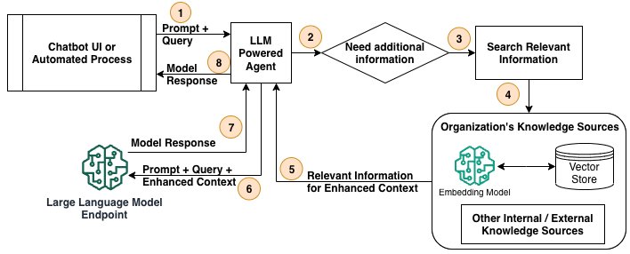
In this post, we dive deep into the vector database options available as part of Amazon Bedrock Knowledge Bases and the applicable use cases, and look at working code examples.
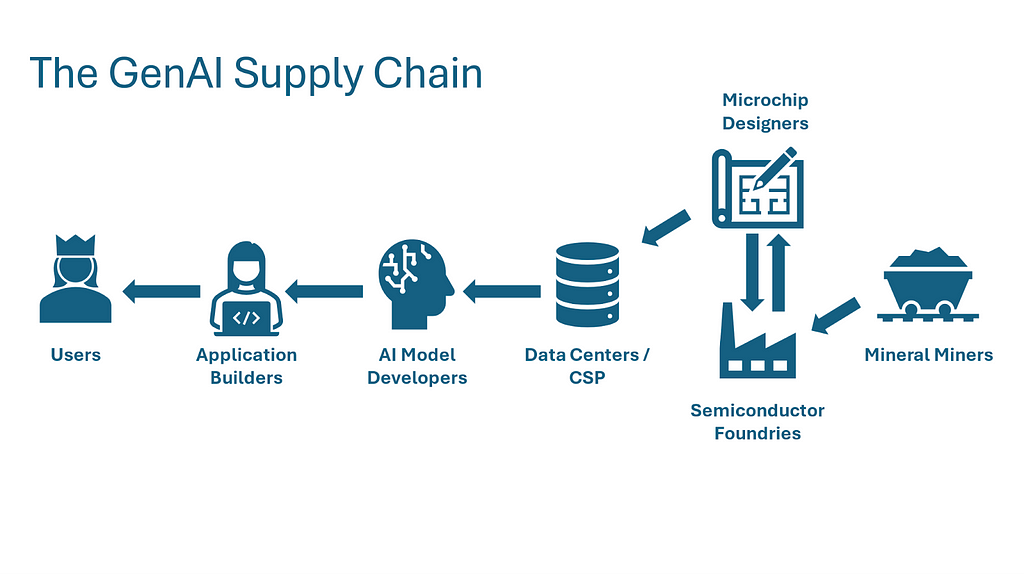
You’ve heard of OpenAI and Nvidia, but do you know who else is involved in the AI wave and how they all fit together?
Image by the author
Several months ago, I visited the MoMA in NYC and saw the work Anatomy of an AI System by Kate Crawford and Vladan Joler. The work examines the Amazon Alexa supply chain from raw resource extraction to devise disposal. This made me to think about everything that goes into producing today’s generative AI (GenAI) powered applications. By digging into this question, I came to understand the many layers of physical and digital engineering that GenAI applications are built upon.
I’ve written this piece to introduce readers to the major components of the GenAI value chain, what role each plays, and who the major players are at each stage. Along the way, I hope to illustrate the range of businesses powering the growth of AI, how different technologies build upon each other, and where vulnerabilities and bottlenecks exist. Starting with the user-facing applications emerging from technology giants like Google and the latest batch of startups, we’ll work backward through the value chain down to the sand and rare earth metals that go into computer chips.
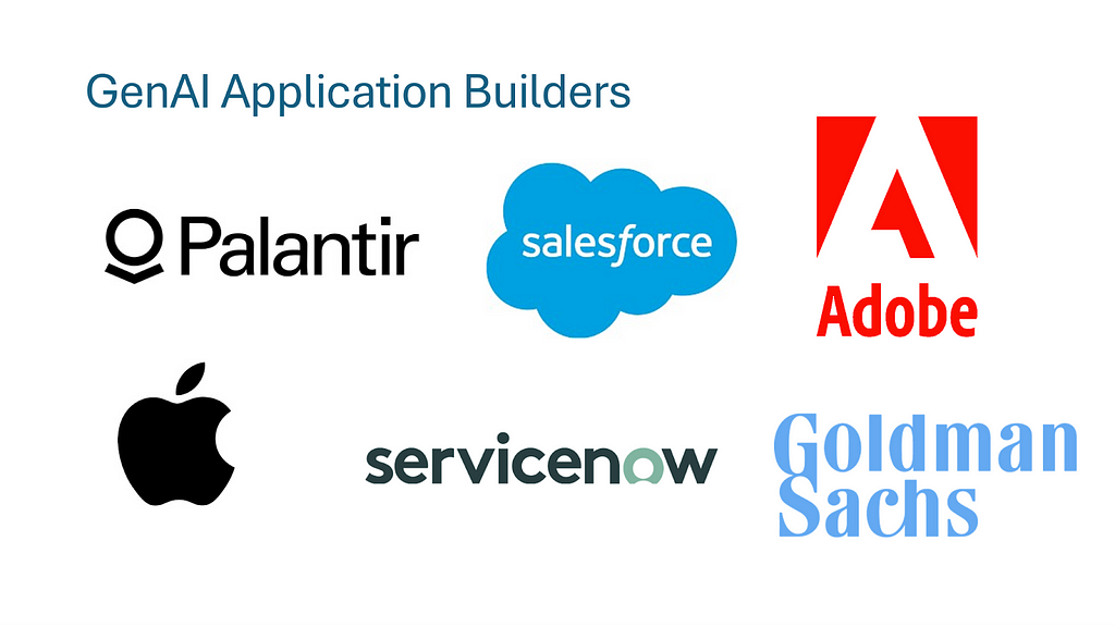
End Application Builders
From scaled startups like Palantir to tech giants like Apple and non-technology companies like Goldman Sachs, everyone is developing AI solutions. Image by the author.
Technology giants, corporate IT departments, and legions of new startups are in the early phases of experimenting with potential use cases for GenAI. These applications may be the start of a new paradigm in computer applications, marked by radical new systems of human-computer interaction and unprecedented capabilities to understand and leverage unstructured and previously untapped data sources (e.g., audio).
Many of the most impactful advances in computing have come from advances in human-computer interaction (HCI). From the development of the GUI to the mouse to the touch screen, these advances have greatly expanded the leverage users gain from computing tools. GenAI models will further remove friction from this interface by equipping computers with the power and flexibility of human language. Users will be able to issue instructions and tasks to computers just as they might a reliable human assistant. Some examples of products innovating in the HCI space are:
Siri (AI Voice Assistant) — Enhances Apple’s mobile assistant with the capability to understand broader requests and questions
Palantir’s AIP (Autonomous Agents) — Strips complexity from large powerful tools through a chat interface that directs users to the desired functionality and actions
Lilac Labs (Customer Service Automation) — Automates drive-through customer ordering with voice AI
GenAI equips computer systems with agency and flexibility that was previously impossible when sets of preprogrammed procedures guided their functionality and their data inputs needed to fit well-defined rules established by the programmer. This flexibility allows applications to perform more complex and open ended knowledge tasks that were previously strictly in the human domain. Some examples of new applications leveraging this flexibility are:
GitHub Copilot (Coding Assistant) — Amplifies programmer productivity by implementing code based on the user’s intent and existing code base
LenAI (Knowledge Assistant) — Saves knowledge workers time by summarizing meetings, extracting critical insights from discussions, and drafting communications
Perplexity (AI Search) — Answers user questions reliably with citations by synthesizing traditional internet searches with AI-generated summaries of internet sources
A diverse group of players is driving the development of these use cases. Hordes of startups are springing up, with 86 of Y Combinator’s W24 batch focused on AI technologies. Major tech companies like Google have also introduced GenAI products and features. For instance, Google is leveraging its Gemini LLM to summarize results in its core search products. Traditional enterprises are launching major initiatives to understand how GenAI can complement their strategy and operations. JP Morgan CEO Jamie Dimon said AI is “unbelievable for marketing, risk, fraud. It’ll help you do your job better.” As companies understand how AI can solve problems and drive value, use cases and demand for GenAI will multiply.
AI Model Builders
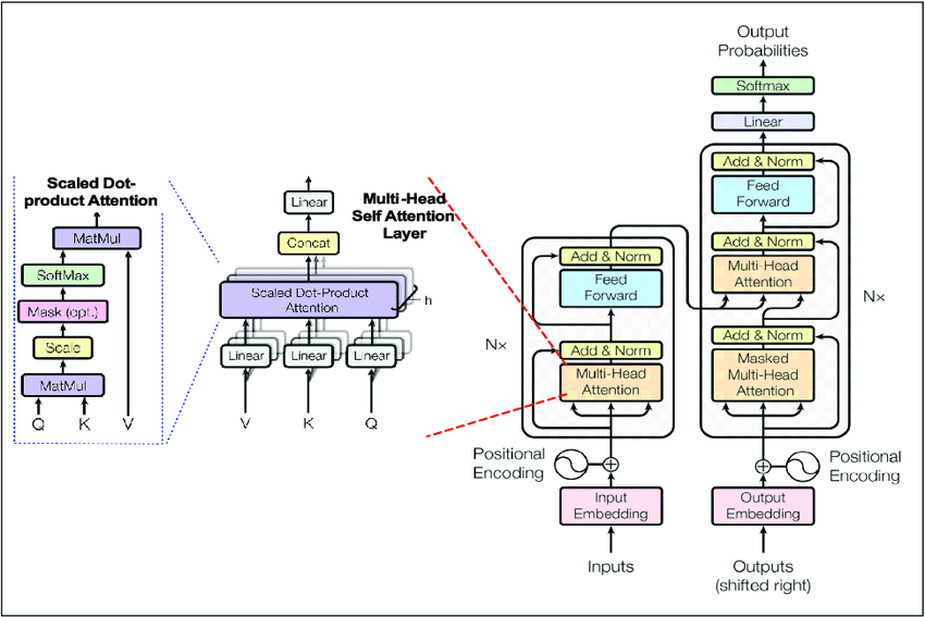
Illustration of the transformer AI architecture. Image by Sing et. al used under Creative Commons 4.0 license.
With the release of OpenAI’s ChatGPT (powered by the GPT-3.5 model) in late 2022, GenAI exploded into the public consciousness. Today, models like Claude (Anthropic), Gemini (Google), and Llama (Meta) have challenged GPT for supremacy. The model provider market and development landscape are still in their infancy, and many open questions remain, such as:
Will smaller domain/task-specific models proliferate, or will large models handle all tasks?
How far can model sophistication and capability advance under the current transformer architecture?
How will capabilities advance as model training approaches the limit of all human-created text data?
Which players will challenge the current supremacy of OpenAI?
While speculating about the capability limits of artificial intelligence is beyond the scope of this discussion, the market for GenAI models is likely large (many prominent investors certainly value it highly). What do model builders do to justify such high valuations and so much excitement?
The research teams at companies like OpenAI are responsible for making architectural choices, compiling and preprocessing training datasets, managing training infrastructure, and more. Research scientists in this field are rare and highly valued; with the average engineer at OpenAI earning over $900k. Not many companies can attract and retain people with this highly specialized skillset required to do this work.
Compiling the training datasets involves crawling, compiling, and processing all text (or audio or visual) data available on the internet and other sources (e.g., digitized libraries). After compiling these raw datasets, engineers layer in relevant metadata (e.g., tagging categories), tokenize data into chunks for model processing, format data into efficient training file formats, and impose quality control measures.
While the market for AI model-powered products and services may be worth trillions within a decade, many barriers to entry prevent all but the most well-resourced companies from building cutting-edge models. The highest barrier to entry is the millions to billions of capital investment required for model training. To train the latest models, companies must either construct their own data centers or make significant purchases from cloud service providers to leverage their data centers. While Moore’s law continues to rapidly lower the price of computing power, this is more than offset by the rapid scale up in model sizes and computation requirements. Training the latest cutting-edge models requires billions in data center investment (in March 2024, media reports described an investment of $100B by OpenAI and Microsoft on data centers to train next gen models). Few companies can afford to allocate billions toward training an AI model (only tech giants or exceedingly well-funded startups like Anthropic and Safe Superintelligence).
Finding the right talent is also incredibly difficult. Attracting this specialized talent requires more than a 7-figure compensation package; it requires connections with the right fields and academic communities, and a compelling value proposition and vision for the technology’s future. Existing players’ high access to capital and domination of the specialized talent market will make it difficult for new entrants to challenge their position.
Knowing a bit about the history of the AI model market helps us understand the current landscape and how the market may evolve. When ChatGPT burst onto the scene, it felt like a breakthrough revolution to many, but was it? Or was it another incremental (albeit impressive) improvement in a long series of advances that were invisible outside of the development world? The team that developed ChatGPT built upon decades of research and publicly available tools from industry, academia, and the open-source community. Most notable is the transformer architecture itself — the critical insight driving not just ChatGPT, but most AI breakthroughs in the past five years. First proposed by Google in their 2017 paper Attention is All You Need, the transformer architecture is the foundation for models like Stable Diffusion, GPT-4, and Midjourney. The authors of that 2017 paper have founded some of the most prominent AI startups (e.g., CharacterAI, Cohere).
Given the common transformer architecture, what will enable some models to “win” against others? Variables like model size, input data quality/quantity, and proprietary research differentiate models. Model size has shown to correlate with improved performance, and the best funded players could differentiate by investing more in model training to further scale up their models. Proprietary data sources (such as those possessed by Meta from its user base and Elon Musk’s xAI from Tesla’s driving videos) could help some models learn what other models don’t have access to. GenAI is still a highly active area of ongoing research — research breakthroughs at companies with the best talent will partially determine the pace of advancement. It’s also unclear how strategies and use cases will create opportunities for different players. Perhaps application builders leverage multiple models to reduce dependency risk or to align a model’s unique strengths with specific use cases (e.g., research, interpersonal communications).
Cloud Service Providers & Data Center Operators
Cloud infrastructure market share. Image by Statistica licensed under Creative Commons.
We discussed how model providers invest billions to build or rent computing resources to train these models. Where is that spending going? Much of it goes to cloud service providers like Microsoft’s Azure (used by OpenAI for GPT) and Amazon Web Services (used by Anthropic for Claude).
Cloud service providers (CSPs) play a crucial role in the GenAI value chain by providing the necessary infrastructure for model training (they also often provide infrastructure to the end application builders, but this section will focus on their interactions with the model builders). Major model builders primarily do not own and operate their own computing facilities (known as data centers). Instead, they rent vast amounts of computing power from the hyper-scaler CSPs (AWS, Azure, and Google Cloud) and other providers.
CSPs produce the resource computing power (manufactured by inputting electricity to a specialized microchip, thousands of which comprise a data center). To train their models, engineers provide the computers operated by CSPs with instructions to make computationally expensive matrix calculations over their input datasets to calculate billions of parameters of model weights. This model training phase is responsible for the high upfront cost of investment. Once these weights are calculated (i.e., the model is trained), model providers use these parameters to respond to user queries (i.e., make predictions on a novel dataset). This is a less computationally expensive process known as inference, also done using CSP computing power.
The cloud service provider’s role is building, maintaining, and administering data centers where this “computing power” resource is produced and used by model builders. CSP activities include acquiring computer chips from suppliers like Nvidia, “racking and stacking” server units in specialized facilities, and performing regular physical and digital maintenance. They also develop the entire software stack to manage these servers and provide developers with an interface to access the computing power and deploy their applications.
The principal operating expense for data centers is electricity, with AI-fueled data center expansion likely to drive a significant increase in electricity usage in the coming decades. For perspective, a standard query to ChatGPT uses ten times as much energy as an average Google Search. Goldman Sachs estimates that AI demand will double the data center’s share of global electricity usage by the decade’s end. Just as significant investments must be made in computing infrastructure to support AI, similar investments must be made to power this computing infrastructure.
Looking ahead, cloud service providers and their model builder partners are in a race to construct the largest and most powerful data centers capable of training the next generation models. The data centers of the future, like those under development by the partnership of Microsoft and OpenAI, will require thousands to millions of new cutting-edge microchips. The substantial capital expenditures by cloud service providers to construct these facilities are now driving record profits at the companies that help build those microchips, notably Nvidia (design) and TSMC (manufacturing).
At this point, everyone’s likely heard of Nvidia and its meteoric, AI-fueled stock market rise. It’s become a cliche to say that the tech giants are locked in an arms race and Nvidia is the only supplier, but is it true? For now, it is. Nvidia designs a form of computer microchip known as a graphical processing unit (GPU) that is critical for AI model training. What is a GPU, and why is it so crucial for GenAI? Why are most conversations in AI chip design centered around Nvidia and not other microchip designers like Intel, AMD, or Qualcomm?
Graphical processing units (as the name suggests) were initially used to serve the computer graphics market. Graphics for CGI movies like Jurassic Park and video games like Doom require expensive matrix computations, but these computations can be done in parallel rather than in series. Standard computer processors (CPUs) are optimized for fast sequential computation (where the input to one step could be output from a prior step), but they cannot do large numbers of calculations in parallel. This optimization for “horizontally” scaled parallel computation rather than accelerated sequential computation was well-suited for computer graphics, and it also came to be perfect for AI training.
Given GPUs served a niche market until the rise of video games in the late 90s, how did they come to dominate the AI hardware market, and how did GPU makers displace Silicon Valley’s original titans like Intel? In 2012, the program AlexNet won the ImageNet machine learning competition by using Nvidia GPUs to accelerate model training. They showed that the parallel computation power of GPUs was perfect for training ML models because like computer graphics, ML model training relied on highly parallel matrix computations. Today’s LLMs have expanded upon AlexNet’s initial breakthrough to scale up to quadrillions of arithmetic computations and billions of model parameters. With this explosion in parallel computing demand since AlexNet, Nvidia has positioned itself as the only potential chip for machine learning and AI model training thanks to heavy upfront investment and clever lock-in strategies.
Given the huge marketing opportunity in GPU design, it is reasonable to ask why Nvidia has no significant challengers (at the time of this writing, Nvidia holds 70–95% of the AI chip market share). Nvidia’s early investments in the ML and AI market before ChatGPT and before even AlexNet were key in establishing a hefty lead over other chipmakers like AMD. Nvidia allocated significant investment in research and development for the scientific computing (to become ML and AI) market segment before there was a clear commercial use case. Because of these early investments, Nvidia had already developed the best supplier and customer relationships, engineering talent, and GPU technology when the AI market took off.
Perhaps Nvidia’s most significant early investment and now its deepest moat against competitors is its CUDA programming platform. CUDA is a low-level software tool that enables engineers to interface with Nvidia’s chips and write parallel native algorithms. Many models, such as LlaMa, leverage higher-level Python libraries built upon these foundational CUDA tools. These lower level tools enable model designers to focus on higher-level architecture design choices without worrying about the complexities of executing calculations at the GPU processor core level. With CUDA, Nvidia built a software solution to strategically complement their hardware GPU products by solving many software challenges AI builders face.
CUDA not only simplifies the process of building parallelized AI and machine learning models on Nvidia chips, it also locks developers onto the Nvidia system, raising significant barriers to exit for any companies looking to switch to Nvidia’s competitors. Programs written in CUDA cannot run on competitor chips, which means that to switch off Nvidia chips, companies must rebuild not just the functionality of the CUDA platform, they must also rebuild any parts of their tech stack dependent on CUDA outputs. Given the massive stack of AI software built upon CUDA over the past decade, there is a substantial switching cost for anyone looking to move to competitors’ chips.
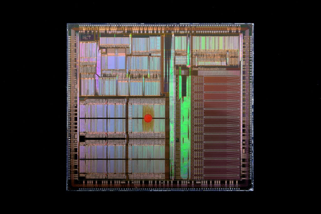
Companies like Nvidia and AMD design chips, but they do not manufacture them. Instead, they rely on semiconductor manufacturing specialists known as foundries. Modern semiconductor manufacturing is one of the most complex engineering processes ever invented, and these foundries are a long way from most people’s image of a traditional factory. To illustrate, transistors on the latest chips are only 12 Silicon atoms long, shorter than the wavelength of visible light. Modern microchips have trillions of these transistors packed onto small silicon wafers and etched into atom-scale integrated circuits.
The key to manufacturing semiconductors is a process known as photolithography. Photolithography involves etching intricate patterns on a silicon wafer, a crystalized form of the element silicon used as the base for the microchip. The process involves coating the wafer with a light-sensitive chemical called photoresist and then exposing it to ultraviolet light through a mask that contains the desired circuit. The exposed areas of the photoresist are then developed, leaving a pattern that can be etched into the wafer. The most critical machines for this process are developed by the Dutch company ASML, which produces extreme ultraviolet (EUV) lithography systems and holds a similar stranglehold to Nvidia in its segment of the AI value chain.
Just as Nvidia came to dominate the GPU design market, its primary manufacturing partner, Taiwan Semiconductor Manufacturing Company (TSMC), holds a similarly large share of the manufacturing market for the most advanced AI chips. To understand TSMC’s place in the semiconductor manufacturing landscape, it is helpful to understand the broader foundry landscape.
Semiconductor manufacturers are split between two main foundry models: pure-play and integrated. Pure-play foundries, such as TSMC and GlobalFoundries, focus exclusively on manufacturing microchips for other companies without designing their own chips (the complement to fabless companies like Nvidia and AMD, who design but do not manufacture their chips). These foundries specialize in fabrication services, allowing fabless semiconductor companies to design microchips without heavy capital expenditures in manufacturing facilities. In contrast, integrated device manufacturers (IDMs) like Intel and Samsung design, manufacture, and sell their chips. The integrated model provides greater control over the entire production process but requires significant investment in both design and manufacturing capabilities. The pure-play model has gained popularity in recent decades due to the flexibility and capital efficiency it offers fabless designers, while the integrated model continues to be advantageous for companies with the resources to maintain design and fabrication expertise.
It is impossible to discuss semiconductor manufacturing without considering the vital role of Taiwan and the consequent geopolitical risks. In the late 20th century, Taiwan transformed itself from a low-margin, low-skilled manufacturing island into a semiconductor powerhouse, largely due to strategic government investments and a focus on high-tech industries. The establishment and growth of TSMC have been central to this transformation, positioning Taiwan at the heart of the global technology supply chain and leading to the outgrowth of many smaller companies to support manufacturing. However, this dominance has also made Taiwan a critical focal point in the ongoing geopolitical struggle, as China views the island as a breakaway province and seeks greater control. Any escalation of tensions could disrupt the global supply of semiconductors, with far-reaching consequences for the global economy, particularly in AI.
At the most basic level, all manufactured objects are created from raw materials extracted from the earth. For microchips used to train AI models, silicon and metals are their primary constituents. These and the chemicals used in the photolithography process are the primary inputs used by foundries to manufacture semiconductors. While the United States and its allies have come to dominate many parts of the value chain, its AI rival, China, has a firmer grasp on raw metals and other inputs.
The primary ingredient in any microchip is silicon (hence the name Silicon Valley). Silicon is one of the most abundant minerals in the earth’s crust and is commonly mined as Silica Dioxide (i.e., quartz or silica sand). Producing silicon wafers involves mining mineral quartzite, crushing it, and then extracting and purifying the elemental silicon. Next, chemical companies such as Sumco and Shin-Etsu Chemical convert pure silicon to wafers using a process called Czochralski growth, in which a seed crystal is dipped into molten high-purity silicon and slowly pulled upwards while rotating. This process creates a sizeable single-crystal silicon ingot sliced into thin wafers, which form the substrate for semiconductor manufacturing.
Beyond Silicon, computer chips also require trace amounts of rare earth metals. A critical step in semiconductor manufacturing is doping, in which impurities are added to the silicon to control conductivity. Doping is typically done with rare earth metals like Germanium, Arsenic, Gallium, and Copper. China dominates the global rare earth metal production, accounting for over 60% of mining and 85% of processing. Other significant rare earth metals producers include Australia, the United States, Myanmar, and the Democratic Republic of the Congo. The United States’ heavy reliance on China for rare earth metals poses significant geopolitical risks, as supply disruptions could severely impact the semiconductor industry and other high-tech sectors. This dependence has prompted efforts to diversify supply chains and develop domestic rare earth production capabilities in the US and other countries, though progress has been slow due to environmental concerns and the complex nature of rare earth processing.
Conclusion
The physical and digital technology stacks and value chains that support the development of AI are intricate and built upon decades of academic and industrial advances. The value chain encompasses end application builders, AI model builders, cloud service providers, chip designers, chip fabricators, and raw material suppliers, among many other key contributors. While much of the attention has been on major players like OpenAI, Nvidia, and TSMC, significant opportunities and bottlenecks exist at all points along the value chain. Thousands of new companies will be born to solve these problems. While companies like Nvidia and OpenAI might be the Intel and Google of their generation, the personal computing and internet booms produced thousands of other unicorns to fill niches and solve issues that came with inventing a new economy. The opportunities created by the shift to AI will take decades to be understood and realized, much as in personal computing in the 70s and 80s and the internet in the 90s and 00s.
While entrepreneurship and crafty engineering may solve many problems in the AI market, some problems involve far greater forces. No challenge is greater than rising geopolitical tension with China, which owns (or claims to own) most of the raw materials and manufacturing markets. This contrasts with the United States and its allies, who control most downstream phases of the chain, including chip design and model training. The struggle for AI dominance is especially vital because the opportunity unlocked by AI is not just economic but also military. Semi-autonomous weapons systems and cyberwarfare agents leveraging AI capabilities may play decisive roles in conflicts of the coming decades. Modern defense technology startups like Palantir and Anduril already show how AI capabilities can expand battlefield visibility and accelerate decision loops to gain potentially decisive advantage. Given AI’s high potential for disruption to the global order and the delicate balance of power between the United States and China, it is imperative that the two nations seek to maintain a cooperative relationship aimed at mutually beneficial development of AI technology for the betterment of global prosperity. Only by solving problems across the supply chain, from the scientific to the industrial to the geopolitical, can the promise of AI to supercharge humanity’s capabilities be realized.
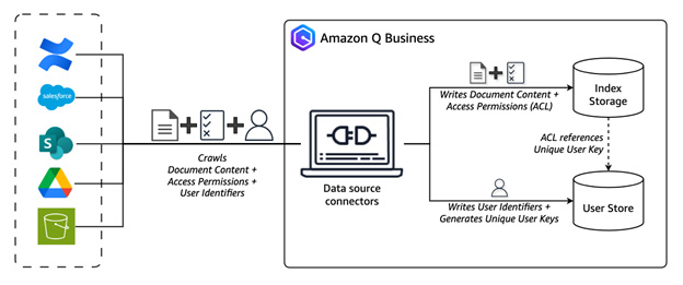
Amazon Q Business recently added support for administrators to modify the default access control list (ACL) crawling feature for data source connectors. Amazon Q Business is a fully managed, AI powered assistant with enterprise-grade security and privacy features. It includes over 40 data source connectors that crawl and index documents. By default, Amazon Q Business […]
A sequence partitioning algorithm that does minimal rearrangements of values
1. Introduction
Sequence partitioning is a basic and frequently used algorithm in computer programming. Given a sequence of numbers “A”, and some value ‘p’ called pivot value, the purpose of a partitioning algorithm is to rearrange numbers inside “A” in such a way, so that all numbers less than ‘p’ come first, followed by the rest of the numbers.
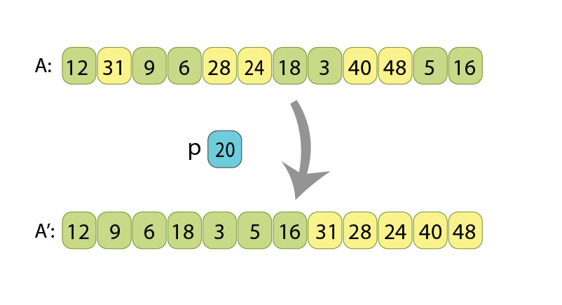
An example of a sequence before and after partitioning by pivot value “p=20”. After the algorithm, all the values which are less than 20 (light green) appear before the other values (yellow).
There are different applications of partitioning, but the most popular are:
QuickSort — which is generally nothing more than a partitioning algorithm, called through recursion multiple times on different sub-arrays of given array, until it becomes sorted.
Finding the median value of a given sequence — which makes use of partitioning in order to efficiently cut down the search range, and to ultimately find the median in expected linear time.
Sorting a sequence is an essential step to enable faster navigation over large amounts of data. Of the two common searching algorithms — linear search and binary search — the latter can only be used if the data in the array is sorted. Finding the median or k’th order statistic can be essential to understand the distribution of values in given unsorted data.
Currently there are different partitioning algorithms (also called — partition schemes), but the well-known ones are “Lomuto scheme” and “Hoare scheme”. Lomuto scheme is often intuitively easier to understand, while Hoare scheme does less rearrangements inside a given array, which is why it is often preferred in practice.
What I am going to suggest in this story is a new partition scheme called “cyclic partition”, which is similar to Hoare scheme, but does 1.5 times fewer rearrangements (value assignments) inside the array. Thus, as it will be shown later, the number of value assignments becomes almost equal to the number of the values which are initially “not at their place”, and should be somehow moved. That fact allows me to consider this new partition scheme as a nearly optimal one.
The next chapters are organized in the following way:
In chapter 2 we will recall what is in-place partitioning (a property, which makes partitioning to be not a trivial task),
In chapter 3 we will recall the widely used Hoare partitioning scheme,
In chapter 4 I’ll present “cycles of assignments”, and we will see why some rearrangements of a sequence might require more value assignments, than other rearrangements of the same sequence,
Chapter 5 will use some properties of “cycles of assignments”, and derive the new “cyclic partition” scheme, as an optimized variant of Hoare scheme,
And finally, chapter 6 will present an experimental comparison between the Hoare scheme and cyclic partition, for arrays of small and large data types.
An implementation of Cyclic partition in the C++ language, as well as its benchmarking with the currently standard Hoare scheme, are present on GitHub, and are referenced at the end of this story [1].
2. Recalling in-place sequence partitioning
Partitioning a sequence will not be a difficult task, if the input and output sequences would reside in computer memory in 2 different arrays. If that would be the case, then one of methods might be to:
Calculate how many values in “A” are less than ‘p’ (this will give us final length of the left part of output sequence),
Scan the input array “A” from left to right, and append every current value “A[i]” either to the left part or to the right part, depending on whether it is less than ‘p’ or not.
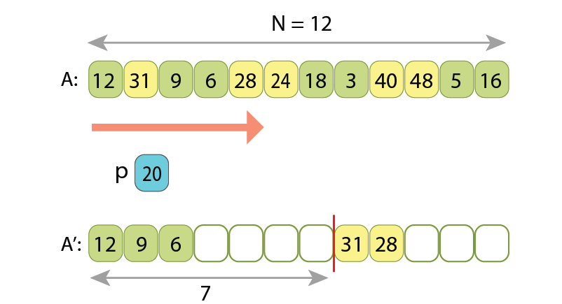
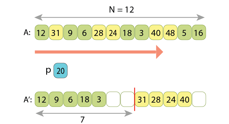
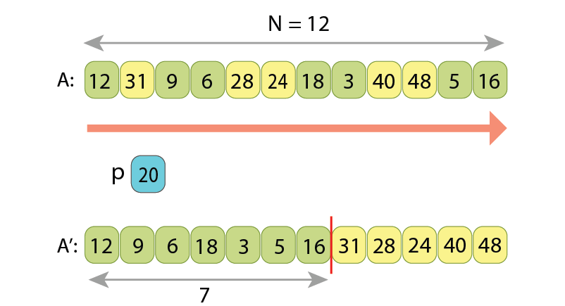
Here are presented a few states of running such algorithm:
During the first stage we calculate that there are only 7 values less than “p=20” (the light green ones), so we prepare to write the greater values into the output sequence, starting from index 7.During the second stage, after scanning 5 values of the input sequence, we append 3 of them to the left part of output sequence, and the other 2 to its right part.Continuing the second stage, we have scanned now 9 values from input sequence, placing 5 of them in the left part of output sequence, and the other 4 to its right part.The algorithm is completed. Both parts of the output sequence are now properly filled to the end. Note, the relative order of values in either left or right parts is preserved, upon how they were originally written in the input array.
Other, shorter solutions also exist, such ones which have only one loop in the code.
Now, the difficulty comes when we want to not use any extra memory, so the input sequence will be transformed into the partitioned output sequence just by moving values inside the only array. By the way, such kind of algorithms which don’t use extra memory are called in-place algorithms.
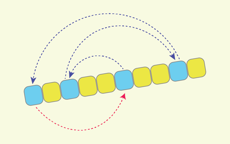
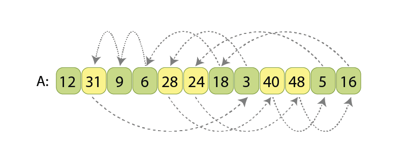
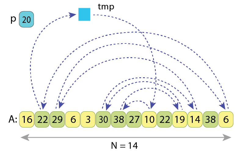
Partitioning the same input sequence “A” in-place, by the same pivot value “p=20”. Presented order of values corresponds to the input state of the sequence, and arrows for every value show if where to that value should be moved, in order for the entire sequence to become partitioned.
Before introducing my partitioning scheme, let’s review the existing and commonly used solution of in-place partitioning.
3. The currently used partitioning scheme
After observing a few implementations of sorting in standard libraries of various programming languages, it looks like the most widely used partitioning algorithm is the Hoare scheme. I found out that it is used for example in:
“std::sort()” implementation in STL for C++,
“Arrays.sort()” implementation in JDK for Java, for primitive data types.
In the partitioning based on the Hoare scheme, we scan the sequence simultaneously from both ends towards each other, searching in the left part such a value A[i] which is greater or equal to ‘p’, and searching in the right part such a value A[j] which is less than ‘p’. Once found, we know that those two values A[i] and A[j] are kind of “not at their proper places” (remember, the partitioned sequence should have the values less than ‘p’ coming first, and only then all the other values which are greater or equal to ‘p’), so we just swap A[i] and A[j]. After the swap, we continue the same way, simultaneously scanning array “A” with indexes i and j, until they become equal. Once they are, partitioning is completed.
Let’s observe the Hoare scheme on another example:
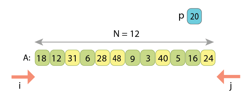
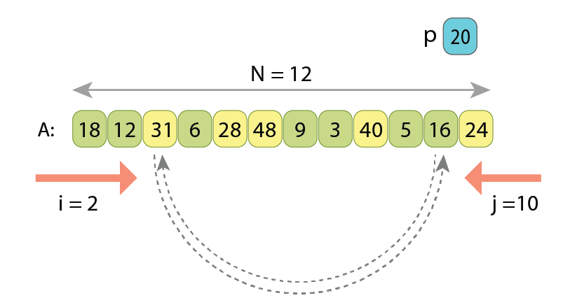
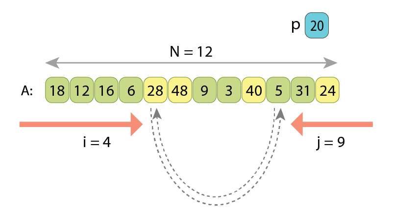
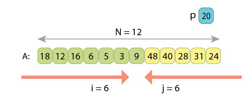
The input sequence “A” of length ’N’, that should be partitioned by pivot value “p=20”. Index i starts scanning from 0 upwards, and index j starts scanning from “N-1” downwards.While increasing index i we meet value “A[2]=31” which is greater than ‘p’. Then, after decreasing index j we meet another value “A[10]=16” which is less than ‘p’. Those 2 are going to be swapped.After swapping “A[2]” and “A[10]” we continue increasing i from 2 and decreasing j from 10. Index i will stop on value “A[4]=28” which is greater than ‘p’, and index j will stop on value “A[9]=5” which is less than ‘p’. Those 2 are also going to be swapped.The algorithm continues the same way, and the numbers “A[5]=48” and “A[7]=3” are also going to be swapped.After that, indexes ‘i’ and ‘j’ will become equal to each other. Partitioning is completed.
If writing the pseudo-code of partitioning by the Hoare scheme, we will have the following:
// Partitions sequence A[0..N) with pivot value 'p'
// upon Hoare scheme, and returns index of the first value
// of the resulting right part.
function partition_hoare( A[0..N) : Array of Integers, p: Integer ) : Integer
    i := 0
    j := N-1
    while true
        // Move left index 'i', as much as needed
        while i < j and A[i] < p
            i := i+1
        // Move right index 'j', as much as needed
        while i < j and A[j] >= p
            j := j-1
        // Check for completion
        if i >= j
            if i == j and A[i] < p
                return i+1  // "A[i]" also refers to left part
            else
                return i  // "A[i]" refers to right part
        // Swap "A[i]" and "A[j]"
        tmp := A[i]
        A[i] := A[j]
        A[j] := tmp
        // Advance by one both 'i' and 'j'
        i := i+1
        j := j-1
Here in lines 5 and 6 we set up start indexes for the 2 scans.
Lines 8–10 search from left for such a value, which should belong to the right part, after partitioning.
Similarly, lines 11–13 search from right for such a value, which should belong to the left part.
Lines 15–19 check for completion of the scans. Once indexes ‘i’ and ‘j’ meet, there are 2 cases: either “A[i]” belongs to the left part or to the right part. Depending on that, we return either ‘i’ or ‘i+1’, as return value of the function should be the start index of the right part.
Next, if the scans are not completed yet, lines 20–23 do swap those 2 values which are not at their proper places.
And finally, lines 24–26 advance the both indexes, in order to not re-check the already swapped values.
The time complexity of the algorithm is O(N), regardless of where the 2 scans will meet each other, as together they always scan N values.
An important note here, if the array “A” has ‘L’ values which are “not at their places”, and should be swapped, then acting by Hoare scheme we will do “3*L/2” assignments, because swapping 2 values requires 3 assignments:
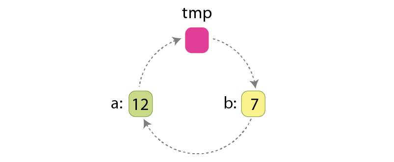
Swapping values of 2 variables ‘a’ and ‘b’ requires to do 3 assignments, with help of ‘tmp’ variable.
Those assignments are:
tmp := a
a := b
b := tmp
Let me also emphasize here that ‘L’ is always an even number. That is because for every value “A[i]>=p” originally residing at the left area, there is another value “A[j]<p” originally residing at the right area, the ones which are being swapped. So, every swap rearranges 2 such values, and all rearrangements in Hoare scheme are being done only through swaps. That’s why the ‘L’ — the total number of values to be rearranged, is always an even number.
4. Cycles of assignments
This chapter might look as a deviation from the agenda of the story, but actually it isn’t, as we will need the knowledge about cycles of assignments in the next chapter, when optimizing the Hoare partitioning scheme.
Assume that we want to somehow rearrange the order of values in given sequence “A”. This should not necessarily be a partitioning, but any kind of rearrangement. Let me show that some rearrangements require more assignments than some others.
Case #1: Cyclic left-shift of a sequence
How many assignments should be done if we want to cyclic left shift the sequence “A” by 1 position?
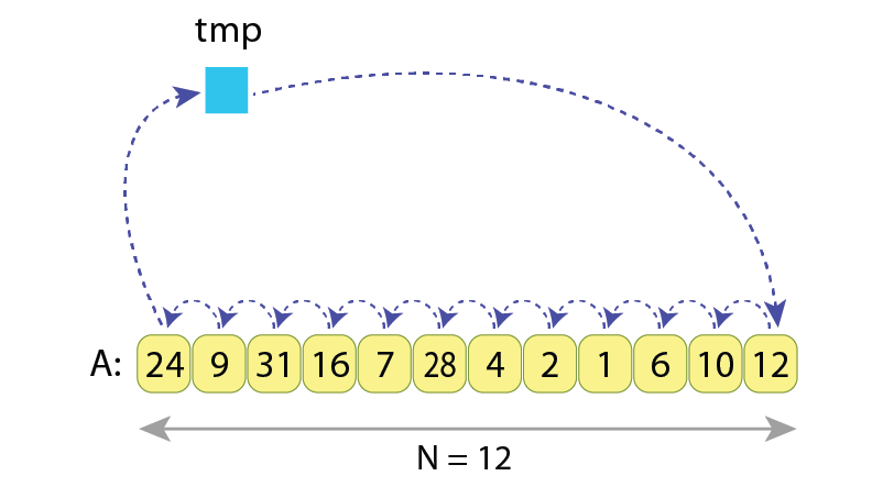
Example of cyclic left shift of sequence “A” of length N=12. We see that the number of assignments needed is N+1=13, as we need to: 1) store “A[0]” in the temporary variable “tmp”, then 2) “N-1” times assign the right adjacent value to the current one, and finally 3) assign “tmp” to the last value of the sequence “A[N-1]”.
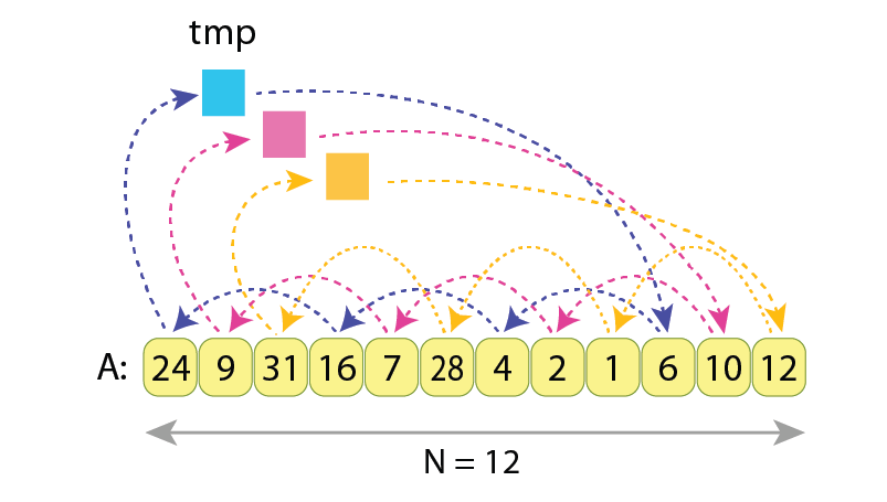
In the next example we still want to do a cyclic left shift of the same sequence, but now by 3 positions to the left:
Example of cyclic left shift by 3 of the sequence “A”, having length N=12. We see that the values A[0], A[3], A[6] and A[9] are being exchanged between each other (blue arrows), as well as values A[1], A[4], A[7] and A[10] do (pink arrows), and as the values A[2], A[5], A[8] and A[11] do exchange only between each other (yellow arrows). The “tmp” variable is being assigned to and read from 3 times.
Here we have 3 independent chains / cycles of assignments, each of length 4.
In order to properly exchange values between A[0], A[3], A[6] and A[9], the needed actions are:
… which makes 5 assignments. Similarly, exchanging values inside groups (A[1], A[4], A[7], A[10]) and (A[2], A[5], A[8], A[11]) will require 5 assignments each. And adding all that together gives 5*3=15 assignments required to cyclic left shift by 3 the sequence “A”, having N=12 values.
Case #3: Reversing a sequence
When reversing the sequence “A” of length ’N’, the actions performed are:
swap its first value with the last one, then
swap the second value with the second one from right,
swap the third value with the third one from right,
… and so on.
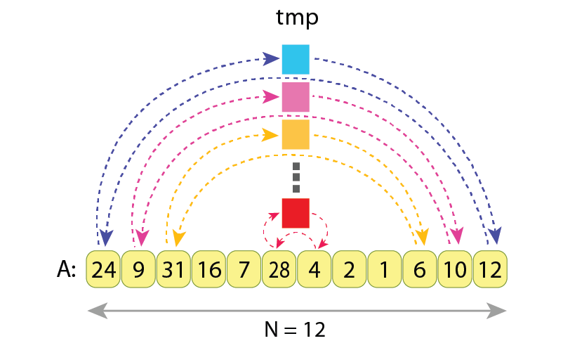
Example of reversing array “A”, having N=12 values. We see that the values in pairs (A[0], A[11]), (A[1], A[10]), (A[2], A[9]), etc, are being swapped, independently from each other. The variable “tmp” is being assigned to and read from 6 times.
As every swap requires 3 assignments, and as for reversing entire sequence “A” we need to do ⌊N/2⌋ swaps, the total number of assignments results in:
3*⌊N/2⌋ = 3*⌊12/2⌋ = 3*6 = 18
And the exact sequence of assignments needed to do the reverse of “A” is:
We have seen that rearranging values of the same sequence “A” might require different number of assignments, depending on how exactly the values are being rearranged.
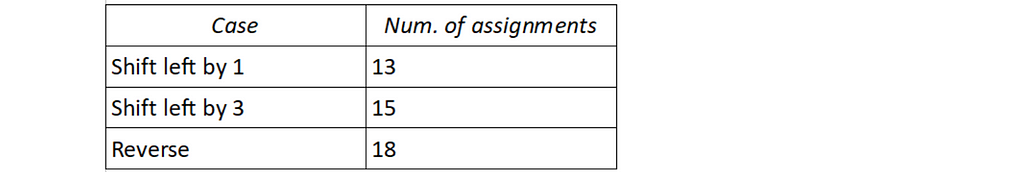
In the presented 3 examples, the sequence always had length of N=12, but the number of required assignments was different:
More precisely, the number of assignments is equal to N+C, where “C” is the number of cycles, which originate during the rearrangement. Here by saying “cycle” I mean such a subset of variables of “A”, values of which are being rotated among each other.
In our case 1 (left shift by 1) we had only C=1 cycle of assignments, and all variables of “A” did participate in that cycle. That’s why overall number of assignments was:
N+C = 12+1 = 13.
In the case 2 (left shift by 3) we had C=3 cycles of assignments, with: — first cycle within variables (A[0], A[3], A[6], A[9]), — second cycle applied to variables (A[1], A[4], A[7], A[10]) and — third cycle applied to variables (A[2], A[5], A[8], A[11]).
That’s why the overall number of assignments was:
N+C = 12+3 = 15.
And in our case 3 (reversing) we had ⌊N/2⌋ = 12/2 = 6 cycles. Those all were the shortest possible cycles, and were applied to pairs (A[0], A[11]), (A[1], A[10]), … and so on. That’s why the overall number of assignments was:
N+C = 12+6 = 18.
Surely, in the presented examples the absolute difference in number of assignments is very small, and it will not play any role when writing high-performance code. But that is because we were considering a very short array of length “N=12”. For longer arrays, those differences in numbers of assignments will grow proportionally to N.
Concluding this chapter, let’s keep in mind that the number of assignments needed to rearrange a sequence grows together with number of cycles, introduced by such rearrangement. And if we want to have a faster rearrangement, we should try to do it by such a scheme, which has the smallest possible number of cycles of assignments.
5. Optimizing the Hoare partitioning scheme
Now let’s observe the Hoare partitioning scheme once again, this time paying attention to how many cycles of assignments it introduces.
Let’s assume we have the same array “A” of length N, and a pivot value ‘p’ according to which the partitioning must be made. Also let’s assume that there are ‘L’ values in the array which should be somehow rearranged, in order to bring “A” into a partitioned state. It turns out that Hoare partitioning scheme rearranges those ‘L’ values in the slowest possible way, because it introduces the maximal possible number of cycles of assignments, with every cycle consisting of only 2 values.
Given pivot value “p=20”, the “L=8” values which should be rearranged are the ones to which arrows are coming (or going from). Hoare partitioning scheme introduces “L/2=4” cycles of assignments, each acting on just 2 values.
Moving 2 values over a cycle of length 2, which is essentially swapping them, requires 3 assignments. So the overall number of values assignments is “3*L/2” for the Hoare partitioning scheme.
The idea which lies beneath the optimization that I am going to describe, comes from the fact that after partitioning a sequence, we are generally not interested in relative order of the values “A[i]<p”, which should finish at the left part of partitioned sequence, as well as we are not interested in the relative order of the ones, which should finish at the right part. The only thing that we are interested in, is for all values less than ‘p’ to come before the other ones. This fact allows us to alter the cycles of assignments in Hoare scheme, and to come up with only 1 cycle of assignments, containing all the ‘L’ values, which should somehow be rearranged.
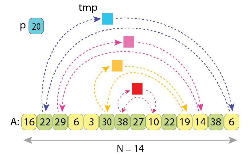
Let me first describe the altered partitioning scheme with the help of the following illustration:
The altered partitioning scheme, applied to the same sequence “A”. As the pivot “p=20” is not changed, the “L=8” values which should be rearranged are also the same. All the arrows represent the only cycle of assignments in the new scheme. After moving all the ‘L’ values upon it, we will end up with an alternative partitioned sequence.
So what are we doing here?
As in the original Hoare scheme, at first we scan from the left and find such value “A[i]>=p” which should go to the right part. But instead of swapping it with some other value, we just remember it: “tmp := A[i]”.
Next we scan from right and find such value “A[j]<p” which should go to the left part. And we just do the assignment “A[i] := A[j]”, without loosing the value of “A[i]”, as it is already stored in “tmp”.
Next we continue the scan from left, and find such value “A[i]>=p” which also should go to the right part. So we do the assignment “A[j] := A[i]”, without loosing value “A[j]”, as it is already assigned to the previous position of ‘i’.
This pattern continues, and once indexes i and j meet each other, it remains to place some value greater than ‘p’ to “A[j]”, we just do “A[j] := tmp”, as initially the variable “tmp” was holding the first value from left, greater than ‘p’. The partitioning is completed.
As we see, here we have only 1 cycle of assignments which goes over all the ‘L’ values, and in order to properly rearrange them it requires just “L+1” value assignments, compared to the “3*L/2” assignments of Hoare scheme.
I prefer to call this new partitioning scheme a “Cyclic partition”, because all the ‘L’ values which should be somehow rearranged, now reside on a single cycle of assignments.
Here is the pseudo-code of the Cyclic partition algorithm. Compared to the pseudo-code of Hoare scheme the changes are insignificant, but now we always do 1.5x fewer assignments.
// Partitions sequence A[0..N) with pivot value 'p'
// by "cyclic partition" scheme, and returns index of
// the first value of the resulting right part.
function partition_cyclic( A[0..N) : Array of Integers, p: Integer ) : Integer
    i := 0
    j := N-1
    // Find the first value from left, which is not on its place
    while i < N and A[i] < p
        i := i+1
    if i == N
        return N  // All N values go to the left part
    // The cycle of assignments starts here
    tmp := A[i]  // The only write to 'tmp' variable
    while true
        // Move right index 'j', as much as needed
        while i < j and A[j] >= p
            j := j-1
        if i == j  // Check for completion of scans
            break
        // The next assignment in the cycle
        A[i] := A[j]
        i := i+1
        // Move left index 'i', as much as needed
        while i < j and A[i] < p
            i := i+1
        if i == j  // Check for completion of scans
            break
        // The next assignment in the cycle
        A[j] := A[i]
        j := j-1
    // The scans have completed
    A[j] := tmp  // The only read from 'tmp' variable
    return j
Here lines 5 and 6 set up the start indexes for both scans (‘i’ — from left to right, and ‘j’ — from right to left).
Lines 7–9 search from left for such a value “A[i]”, which should go to the right part. If it turns out that there is no such value, and all N items belong to the left part, lines 10 and 11 report that and finish the algorithm.
Otherwise, if such value was found, at line 13 we remember it in the ‘tmp’ variable, thus opening a slot at index ‘i’ for placing another value there.
Lines 15–19 search from right for such a value “A[j]” which should be moved to the left part. Once found, lines 20–22 place it into the empty slot at index ‘i’, after which the slot at index ‘j’ becomes empty, and waits for another value.
Similarly, lines 23–27 search from left for such a value “A[i]” which should be moved to the right part. Once found, lines 28–30 place it into the empty slot at index ‘j’, after which the slot at index ‘i’ again becomes empty, and waits for another value.
This pattern is continued in the main loop of the algorithm, at lines 14–30.
Once indexes ‘i’ and ‘j’ meet each other, we have an empty slot there, and lines 31 and 32 assign the originally remembered value in ‘tmp’ variable there, so the index ‘j’ becomes the first one to hold such value which belongs to the right part.
The last line returns that index.
This way we can write 2 assignments of the cycle together in the loop’s body, because as it was proven in chapter 3, ‘L’ is always an even number.
Time complexity of this algorithm is also O(N), as we still scan the sequence from both ends. It just does 1.5x less value assignments, so the speed-up is reflected only in the constant factor.
An implementation of Cyclic partition in the C++ language is present on GitHub, and is referenced at the end of this story [1].
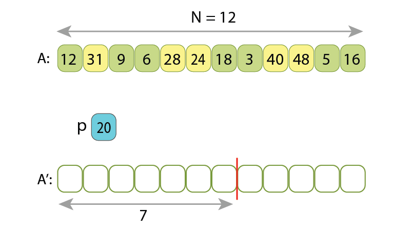
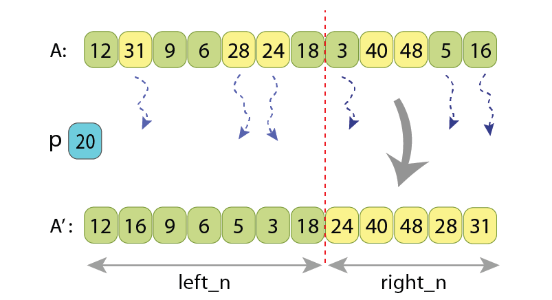
I also want to show that the value ‘L’ figuring in the Hoare scheme can’t be lowered, regardless of what partitioning scheme we use. Assume that after partitioning, the length of the left part will be “left_n”, and length of the right part will be “right_n”. Now, if looking at the left-aligned “left_n”-long area of the original unpartitioned array, we will find some ‘t1’ values there, which are not at their final places. So those are such values which are greater or equal to ‘p’, and should be moved to the right part anyway.
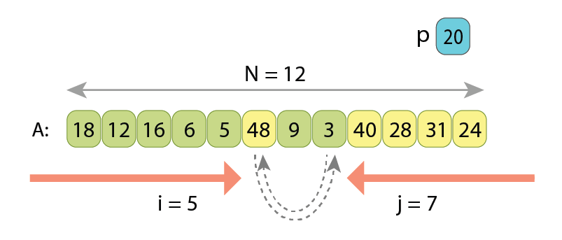
Illustration of the sequence before and after partitioning. Length of the left part is “left_n=7” and length of the right part is “right_n=5”. Among the first 7 values of the unpartitioned sequence there are “t1=3” of them which are greater than “p=20” (the yellow ones), and should be somehow moved to the right part. And among the last 5 values of the unpartitioned sequence there are “t2=3” of them which are less than ‘p’ (the light green ones), and should be somehow moved to the left part.
Similarly, if looking at the right-aligned “right_n”-long area of the original unpartitioned array, we will find some ‘t2’ values there, which are also not at their final places. Those are such values which are less than ‘p’, and should be moved to the left part. We can’t move less than ‘t1’ values from left to right, as well as we can’t move less than ‘t2’ values from right to left.
In the Hoare partitioning scheme, the ‘t1’ and ‘t2’ values are the ones which are swapped between each other. So there we have:
t1 = t2 = L/2,
or
t1 + t2 = L.
Which means that ‘L’ is actually the minimal amount of values which should be somehow rearranged, in order for the sequence to become partitioned. And the Cyclic partition algorithm rearranges them doing just “L+1” assignments. That’s why I allow myself to call this new partitioning scheme as “nearly optimal”.
6. Experimental results
It is already proven that the new partitioning scheme is doing fewer assignments of values, so we can expect it to run faster. However, before publishing the algorithm I wanted to collect the results also in an experimental way.
I have compared the running times when partitioning by the Hoare scheme and by Cyclic partition. All the experiments were performed on randomly shuffled arrays.
The parameters by which the experiments were different are:
N — length of the array,
“left_part_percent” — percent of length of the left part (upon N), which results after partitioning,
running on array of primitive data type variables (32-bit integers) vs. on array of some kind of large objects (256-long static arrays of 16-bit integers).
I want to clarify why I found it necessary to run partitioning both on arrays of primitive data types, and on arrays of large objects. Here, by saying “large object” I mean such values, which occupy much more memory, compared to primitive data types. When partitioning primitive data types, assigning one variable to another will work as fast as almost all other instructions used in both algorithms (like incrementing an index or checking condition of the loop). Meanwhile when partitioning large objects, assigning one such object to another will take significantly more time, compared to other used instructions, and that is when we are interested to reduce the overall number of value assignments as much as that is possible.
I’ll explain why I decided to run different experiments with different values of “left_part_percent” a bit later in this chapter.
The experiments were performed with Google Benchmark, under the following system:
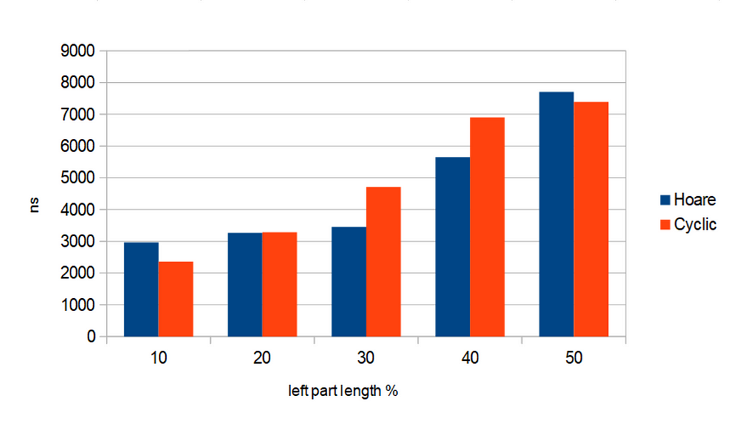
Here are the results of running partition algorithms on arrays of primitive data type — 32 bit integer:
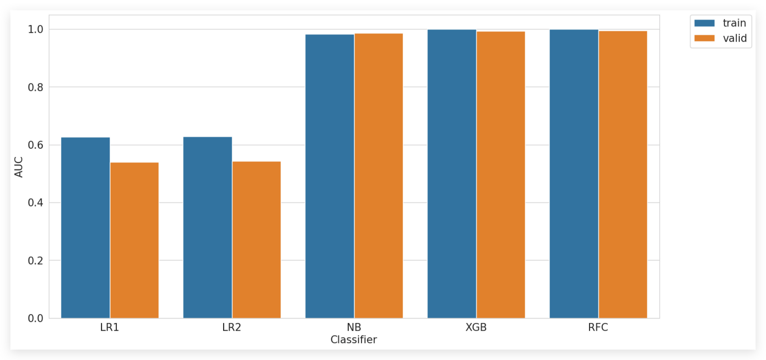
Running times of partitioning algorithms, on array of 32-bit integers, having length N=10’000. Blue bars correspond to partitioning by Hoare scheme, while red bars correspond to the Cyclic partition algorithm. Partitioning algorithms are run for 5 different cases, based on “left_part_percent” — percent of the left part of array (upon N), that will appear after partitioning. The time is presented in nanoseconds.
We see that there is no obvious correlation between value of “left_part_percent” and relative difference in running times of the 2 algorithms. This kind of behavior is expected.
Partitioning arrays of “large objects”
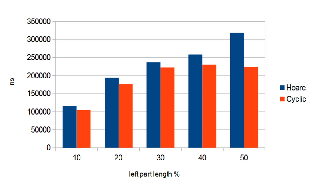
And here are the results of running the 2 partitioning algorithms on array of so called “large objects” — each of which is an 256-long static array of 16-bit random integers.
Running times of partitioning algorithms, on array of large objects (256-long static arrays of random 16-bit integers), having length N=10’000. Blue bars correspond to partitioning by Hoare scheme, while red bars correspond to the Cyclic partition algorithm. Partitioning algorithms are run for 5 different cases, based on “left_part_percent” — percent of the left part of array (upon N), that will appear after partitioning. The time is presented in nanoseconds.
Now we see an obvious correlation: Cyclic partition outperforms the Hoare scheme as more, as the “left_part_percent” is closer to 50%. In other words, Cyclic partition works relatively faster when after partitioning the left and right parts of the array appear to have closer lengths. This is also an expected behavior.
Explanation of the results
— Why does partitioning generally take longer, when “left_part_percent” is closer to 50%?
Let’s imagine for a moment a corner case — when after partitioning almost all values appear in left (or right) part. This will mean that almost all values of the array were less (or greater) than the pivot value. And it will mean that during the scan, all those values were considered to be already at their final positions, and very few assignments of values were performed. If trying to imagine the other case — when after partitioning the left and right parts appear to have almost equal length, it will mean that a lot of value assignments were performed (as initially all the values were randomly shuffled in the array).
— When looking at partitioning of “large objects”, why does the difference in running time of the 2 algorithms become greater when “left_part_percent” gets closer to 50%?
The previous explanation shows that when “left_part_percent” gets closer to 50%, there arises need to do more assignments of values in the array. In previous chapters we also have shown that Cyclic partition always makes 1.5x less value assignments, compared to Hoare scheme. So that difference of 1.5 times brings more impact on overall running time when we generally need to do more rearrangements of values in the array.
— Why is the absolute time (in nanoseconds) greater when partitioning “large objects”, rather than when partitioning 32-bit integers?
This one is simple — because assigning one “large object” to another takes much more time, than assigning one primitive data type to another.
I also run all the experiments on arrays with different lengths, but the overall picture didn’t change.
7. Conclusion
In this story I introduced an altered partitioning scheme, called “Cyclic partition”. It always makes 1.5 times fewer value assignments, compared to the currently used Hoare partitioning scheme.
Surely, when partitioning a sequence, value assignment is not the only type of operation performed. Besides it, partitioning algorithms check values of input sequence “A” for being less or greater than the pivot value ‘p’, as well as they do increments and decrements of indexes over “A”. The amounts of comparisons, increments and decrements are not affected by introducing “cyclic partition”, so we can’t just expect it to run 1.5x faster. However, when partitioning an array of complex data types, where value assignment is significantly more time-consuming than simply incrementing or decrementing an index, the overall algorithm can actually run up to 1.5 times faster.
The partitioning procedure is the main routine of the QuickSort algorithm, as well as of the algorithm for finding the median of an unsorted array, or finding its k-th order statistic. So we can also expect for those algorithms to have a performance gain up to 1.5 times, when working on complex data types.
In this post, we share how SKT customizes Anthropic Claude models for telco-specific Q&A regarding technical telecommunication documents of SKT using Amazon Bedrock.
Originally appeared here:
SK Telecom improves telco-specific Q&A by fine-tuning Anthropic’s Claude models in Amazon Bedrock
SK Telecom improves telco-specific Q&A by fine-tuning Anthropic’s Claude models in Amazon Bedrock
We use cookies on our website to give you the most relevant experience by remembering your preferences and repeat visits. By clicking “Accept”, you consent to the use of ALL the cookies.
This website uses cookies to improve your experience while you navigate through the website. Out of these, the cookies that are categorized as necessary are stored on your browser as they are essential for the working of basic functionalities of the website. We also use third-party cookies that help us analyze and understand how you use this website. These cookies will be stored in your browser only with your consent. You also have the option to opt-out of these cookies. But opting out of some of these cookies may affect your browsing experience.
Necessary cookies are absolutely essential for the website to function properly. These cookies ensure basic functionalities and security features of the website, anonymously.
Cookie
Duration
Description
cookielawinfo-checkbox-analytics
11 months
This cookie is set by GDPR Cookie Consent plugin. The cookie is used to store the user consent for the cookies in the category "Analytics".
cookielawinfo-checkbox-functional
11 months
The cookie is set by GDPR cookie consent to record the user consent for the cookies in the category "Functional".
cookielawinfo-checkbox-necessary
11 months
This cookie is set by GDPR Cookie Consent plugin. The cookies is used to store the user consent for the cookies in the category "Necessary".
cookielawinfo-checkbox-others
11 months
This cookie is set by GDPR Cookie Consent plugin. The cookie is used to store the user consent for the cookies in the category "Other.
cookielawinfo-checkbox-performance
11 months
This cookie is set by GDPR Cookie Consent plugin. The cookie is used to store the user consent for the cookies in the category "Performance".
viewed_cookie_policy
11 months
The cookie is set by the GDPR Cookie Consent plugin and is used to store whether or not user has consented to the use of cookies. It does not store any personal data.
Functional cookies help to perform certain functionalities like sharing the content of the website on social media platforms, collect feedbacks, and other third-party features.
Performance cookies are used to understand and analyze the key performance indexes of the website which helps in delivering a better user experience for the visitors.
Analytical cookies are used to understand how visitors interact with the website. These cookies help provide information on metrics the number of visitors, bounce rate, traffic source, etc.
Advertisement cookies are used to provide visitors with relevant ads and marketing campaigns. These cookies track visitors across websites and collect information to provide customized ads.