Tag: artificial intelligence

Llama-3.2–1 B-Instruct and LanceDB

Abstract: Retrieval-augmented generation (RAG) combines large language models with external knowledge sources to produce more accurate and contextually relevant responses. This article explores how smaller language models (LLMs), like the recently opensourced Meta 1 Billion model, can be effectively utilized to summarize and index large documents, thereby improving the efficiency and scalability of RAG systems. We provide a step-by-step guide, complete with code snippets, on how to summarize chunks of text from a product documentation PDF and store them in a LanceDB database for efficient retrieval.

Introduction

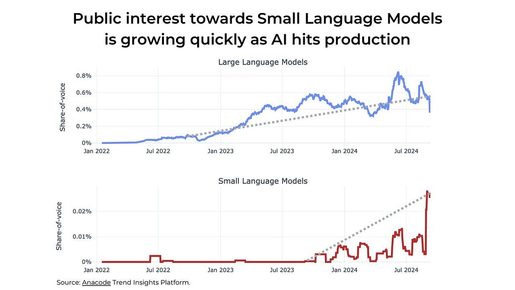
Retrieval-Augmented Generation is a paradigm that enhances the capabilities of language models by integrating them with external knowledge bases. While large LLMs like GPT-4 have demonstrated remarkable capabilities, they come with significant computational costs. Small LLMs offer a more resource-efficient alternative, especially for tasks like text summarization and keyword extraction, which are crucial for indexing and retrieval in RAG systems.

In this article, we’ll demonstrate how to use a small LLM to:

1. Extract and summarize text from a PDF document.
2. Generate embeddings for summaries and keywords.
3. Store the data efficiently in a LanceDB database.
4. Use this for effective RAG
5. Also a Agentic workflow for self correcting errors from the LLM

Using a smaller LLM drastically reduces the cost for these types of conversions on huge data-sets and gets similar benefits for simpler tasks as the larger parameter LLMs and can easily be hosted in the Enterprise or from the Cloud with minimal cost.

We will use LLAMA 3.2 1 Billion parameter model, the smallest state-of-the-art LLM as of now.

The Problem with Embedding Raw Text

Before diving into the implementation, it’s essential to understand why embedding raw text from documents can be problematic in RAG systems.

Ineffective Context Capture

Embedding raw text from a page without summarization often leads to embeddings that are:

• High-dimensional noise: Raw text may contain irrelevant information, formatting artefacts, or boilerplate language that doesn’t contribute to understanding the core content.
• Diluted key concepts: Important concepts may be buried within extraneous text, making the embeddings less representative of the critical information.

Retrieval Inefficiency

When embeddings do not accurately represent the key concepts of the text, the retrieval system may fail to:

• Match user queries effectively: The embeddings might not align well with the query embeddings, leading to poor retrieval of relevant documents.
• Provide correct context: Even if a document is retrieved, it may not offer the precise information the user is seeking due to the noise in the embedding.

Solution: Summarization Before Embedding

Summarizing the text before generating embeddings addresses these issues by:

• Distilling Key Information: Summarization extracts the essential points and keywords, removing unnecessary details.
• Improving Embedding Quality: Embeddings generated from summaries are more focused and representative of the main content, enhancing retrieval accuracy.

Prerequisites

Before we begin, ensure you have the following installed:

• Python 3.7 or higher
• PyTorch
• Transformers library
• SentenceTransformers
• PyMuPDF (for PDF processing)
• LanceDB
• A laptop with GPU Min 6 GB or Colab (T4 GPU will be sufficient) or similar

Step 1: Setting Up the Environment

First, import all the necessary libraries and set up logging for debugging and tracking.

import pandas as pd
import fitz  # PyMuPDF
from transformers import AutoModelForCausalLM, AutoTokenizer
import torch
import lancedb
from sentence_transformers import SentenceTransformer
import json
import pyarrow as pa
import numpy as np
import re

Step 2: Defining Helper Functions

Creating the Prompt

We define a function to create prompts compatible with the LLAMA 3.2 model.

def create_prompt(question):
    """
    Create a prompt as per LLAMA 3.2 format.
    """
    system_message = "You are a helpful assistant for summarizing text and result in JSON format"
    prompt_template = f'''
<|begin_of_text|><|start_header_id|>system<|end_header_id|>
{system_message}<|eot_id|><|start_header_id|>user<|end_header_id|>
{question}<|eot_id|><|start_header_id|>assistant1231231222<|end_header_id|>
'''
    return prompt_template

Processing the Prompt

This function processes the prompt using the model and tokenizer. We are setting the temperature to 0.1 to make the model less creative (less hallucinating)

def process_prompt(prompt, model, tokenizer, device, max_length=500):
    """
    Processes a prompt, generates a response, and extracts the assistant's reply.
    """
    prompt_encoded = tokenizer(prompt, truncation=True, padding=False, return_tensors="pt")
    model.eval()
    output = model.generate(
        input_ids=prompt_encoded.input_ids.to(device),
        max_new_tokens=max_length,
        attention_mask=prompt_encoded.attention_mask.to(device),
        temperature=0.1  # More deterministic
    )
    answer = tokenizer.decode(output[0], skip_special_tokens=True)
    parts = answer.split("assistant1231231222", 1)
   if len(parts) > 1:
        words_after_assistant = parts[1].strip()
        return words_after_assistant
    else:
        print("The assistant's response was not found.")
        return "NONE"

Step 3: Loading the Model

We use the LLAMA 3.2 1B Instruct model for summarization. We are loading the model with bfloat16 to reduce the memory and running in NVIDIA laptop GPU (NVIDIA GeForce RTX 3060 6 GB/ Driver NVIDIA-SMI 555.58.02/Cuda compilation tools, release 12.5, V12.5.40) in a Linux OS.

Better would be to host via vLLM or better exLLamaV2

model_name_long = "meta-llama/Llama-3.2-1B-Instruct"
tokenizer = AutoTokenizer.from_pretrained(model_name_long)
device = torch.device("cuda" if torch.cuda.is_available() else "cpu")
log.info(f"Loading the model {model_name_long}")
bf16 = False
fp16 = True
if torch.cuda.is_available():
    major, _ = torch.cuda.get_device_capability()
    if major >= 8:
        log.info("Your GPU supports bfloat16: accelerate training with bf16=True")
        bf16 = True
        fp16 = False
# Load the model
device_map = {"": 0}  # Load on GPU 0
torch_dtype = torch.bfloat16 if bf16 else torch.float16
model = AutoModelForCausalLM.from_pretrained(
    model_name_long,
    torch_dtype=torch_dtype,
    device_map=device_map,
)
log.info(f"Model loaded with torch_dtype={torch_dtype}")

Step 4: Reading and Processing the PDF Document

We extract text from each page of the PDF document.

file_path = './data/troubleshooting.pdf'
dict_pages = {}
# Open the PDF file
with fitz.open(file_path) as pdf_document:
    for page_number in range(pdf_document.page_count):
        page = pdf_document.load_page(page_number)
        page_text = page.get_text()
        dict_pages[page_number] = page_text
        print(f"Processed PDF page {page_number + 1}")

Step 5: Setting Up LanceDB and SentenceTransformer

We initialize the SentenceTransformer model for generating embeddings and set up LanceDB for storing the data. We are using PyArrow based Schema for the LanceDB tables

Note that keywords are not used now but can be used for hybrid search, that is vector similarity search as well as text search if needed.

# Initialize the SentenceTransformer model
sentence_model = SentenceTransformer('all-MiniLM-L6-v2')
# Connect to LanceDB
db = lancedb.connect('./data/my_lancedb')
# Define the schema using PyArrow
schema = pa.schema([
    pa.field("page_number", pa.int64()),
    pa.field("original_content", pa.string()),
    pa.field("summary", pa.string()),
    pa.field("keywords", pa.string()),
    pa.field("vectorS", pa.list_(pa.float32(), 384)),  # Embedding size of 384
    pa.field("vectorK", pa.list_(pa.float32(), 384)),
])
# Create or connect to a table
table = db.create_table('summaries', schema=schema, mode='overwrite')

Step 6: Summarizing and Storing Data

We loop through each page, generate a summary and keywords, and store them along with embeddings in the database.

# Loop through each page in the PDF
for page_number, text in dict_pages.items():
    question = f"""For the given passage, provide a long summary about it, incorporating all the main keywords in the passage.
Format should be in JSON format like below:
{{
    "summary": <text summary>,
    "keywords": <a comma-separated list of main keywords and acronyms that appear in the passage>,
}}
Make sure that JSON fields have double quotes and use the correct closing delimiters.
Passage: {text}"""
    
    prompt = create_prompt(question)
    response = process_prompt(prompt, model, tokenizer, device)
    
    # Error handling for JSON decoding
    try:
        summary_json = json.loads(response)
    except json.decoder.JSONDecodeError as e:
        exception_msg = str(e)
        question = f"""Correct the following JSON {response} which has {exception_msg} to proper JSON format. Output only JSON."""
        log.warning(f"{exception_msg} for {response}")
        prompt = create_prompt(question)
        response = process_prompt(prompt, model, tokenizer, device)
        log.warning(f"Corrected '{response}'")
        try:
            summary_json = json.loads(response)
        except Exception as e:
            log.error(f"Failed to parse JSON: '{e}' for '{response}'")
            continue
    
    keywords = ', '.join(summary_json['keywords'])
    
    # Generate embeddings
    vectorS = sentence_model.encode(summary_json['summary'])
    vectorK = sentence_model.encode(keywords)
    
    # Store the data in LanceDB
    table.add([{
        "page_number": int(page_number),
        "original_content": text,
        "summary": summary_json['summary'],
        "keywords": keywords,
        "vectorS": vectorS,
        "vectorK": vectorK
    }])
    
    print(f"Data for page {page_number} stored successfully.")

Using LLMs to Correct Their Outputs

When generating summaries and extracting keywords, LLMs may sometimes produce outputs that are not in the expected format, such as malformed JSON.

We can leverage the LLM itself to correct these outputs by prompting it to fix the errors. This is shown in the code above

# Use the Small LLAMA 3.2 1B model to create summary
for page_number, text in dict_pages.items():
    question = f"""For the given passage, provide a long summary about it, incorporating all the main keywords in the passage.
    Format should be in JSON format like below: 
    {{
        "summary": <text summary> example "Some Summary text",
        "keywords": <a comma separated list of main keywords and acronyms that appear in the passage> example ["keyword1","keyword2"],
    }}
    Make sure that JSON fields have double quotes, e.g., instead of 'summary' use "summary", and use the closing and ending delimiters.
    Passage: {text}"""
    prompt = create_prompt(question)
    response = process_prompt(prompt, model, tokenizer, device)
    try:
        summary_json = json.loads(response)
    except json.decoder.JSONDecodeError as e:
        exception_msg = str(e)
        # Use the LLM to correct its own output
        question = f"""Correct the following JSON {response} which has {exception_msg} to proper JSON format. Output only the corrected JSON.
        Format should be in JSON format like below: 
        {{
            "summary": <text summary> example "Some Summary text",
            "keywords": <a comma separated list of keywords and acronyms that appear in the passage> example ["keyword1","keyword2"],
        }}"""
        log.warning(f"{exception_msg} for {response}")
        prompt = create_prompt(question)
        response = process_prompt(prompt, model, tokenizer, device)
        log.warning(f"Corrected '{response}'")
        # Try parsing the corrected JSON
        try:
            summary_json = json.loads(response)
        except json.decoder.JSONDecodeError as e:
            log.error(f"Failed to parse corrected JSON: '{e}' for '{response}'")
            continue

In this code snippet, if the LLM’s initial output cannot be parsed as JSON, we prompt the LLM again to correct the JSON. This self-correction pattern improves the robustness of our pipeline.

Suppose the LLM generates the following malformed JSON:

{
    'summary': 'This page explains the installation steps for the product.',
    'keywords': ['installation', 'setup', 'product']
}

Attempting to parse this JSON results in an error due to the use of single quotes instead of double quotes. We catch this error and prompt the LLM to correct it:

exception_msg = "Expecting property name enclosed in double quotes"
question = f"""Correct the following JSON {response} which has {exception_msg} to proper JSON format. Output only the corrected JSON."""

The LLM then provides the corrected JSON:

{
    "summary": "This page explains the installation steps for the product.",
    "keywords": ["installation", "setup", "product"]
}

By using the LLM to correct its own output, we ensure that the data is in the correct format for downstream processing.

Extending Self-Correction via LLM Agents

This pattern of using the LLM to correct its outputs can be extended and automated through the use of LLM Agents. LLM Agents can:

• Automate Error Handling: Detect errors and autonomously decide how to correct them without explicit instructions.
• Improve Efficiency: Reduce the need for manual intervention or additional code for error correction.
• Enhance Robustness: Continuously learn from errors to improve future outputs.

LLM Agents act as intermediaries that manage the flow of information and handle exceptions intelligently. They can be designed to:

• Parse outputs and validate formats.
• Re-prompt the LLM with refined instructions upon encountering errors.
• Log errors and corrections for future reference and model fine-tuning.

Approximate Implementation:

Instead of manually catching exceptions and re-prompting, an LLM Agent could encapsulate this logic:

def generate_summary_with_agent(text):
    agent = LLMAgent(model, tokenizer, device)
    question = f"""For the given passage, provide a summary and keywords in proper JSON format."""
    prompt = create_prompt(question)
    response = agent.process_and_correct(prompt)
    return response

The LLMAgent class would handle the initial processing, error detection, re-prompting, and correction internally.

Now lets see how we can use the Embeddings for an effective RAG pattern again using the LLM to help in ranking.

Retrieval and Generation: Processing the User Query

This is the usual flow. We take the user’s question and search for the most relevant summaries.

# Example usage
user_question = "Not able to manage new devices"
results = search_summary(user_question, sentence_model)

Preparing the Retrieved Summaries

We compile the retrieved summaries into a list, associating each summary with its page number for reference.

summary_list = []
for idx, result in enumerate(results):
    summary_list.append(f"{result['page_number']}# {result['summary']}")

Ranking the Summaries

We prompt the language model to rank the retrieved summaries based on their relevance to the user’s question and select the most relevant one. This is again using the LLM in ranking the summaries than the K-Nearest Neighbour or Cosine distance or other ranking algorithms alone for the contextual embedding (vector) match.

question = f"""From the given list of summaries {summary_list}, rank which summary would possibly have 
the answer to the question '{user_question}'. Return only that summary from the list."""
log.info(question)

Extracting the Selected Summary and Generating the Final Answer

We retrieve the original content associated with the selected summary and prompt the language model to generate a detailed answer to the user’s question using this context.

for idx, result in enumerate(results):
    if int(page_number) == result['page_number']:
        page = result['original_content']
        question = f"""Can you answer the query: '{user_question}' 
using the context below?
Context: '{page}'
"""
        log.info(question)
        prompt = create_prompt(
            question,
            "You are a helpful assistant that will go through the given query and context, think in steps, and then try to answer the query 
with the information in the context."
        )
        response = process_prompt(prompt, model, tokenizer, device, temperature=0.01)  # Less freedom to hallucinate
        log.info(response)
        print("Final Answer:")
        print(response)
        break

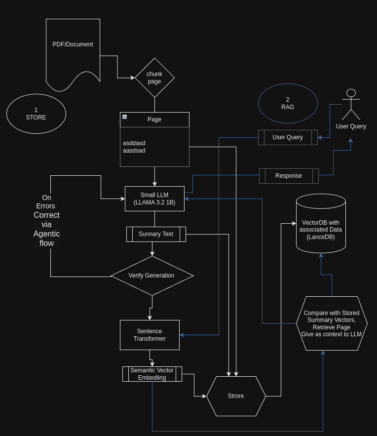
Explanation of the Workflow

1. User Query Vectorization: The user’s question is converted into an embedding using the same SentenceTransformer model used during indexing.
2. Similarity Search: The query embedding is used to search the vector database (LanceDB) for the most similar summaries and return Top 3

>>  From the VectorDB Cosine search and Top 3 nearest neighbour search result, 
prepended by linked page numbers

07:04:00 INFO:From the given list of summary [[
'112# Cannot place newly discovered device in managed state', 
'113# The passage discusses the troubleshooting steps for managing newly discovered devices on the NSF platform, specifically addressing issues with device placement, configuration, and deployment.',
'116# Troubleshooting Device Configuration Backup Issue']] rank which summary would possibly have the possible answer to the question Not able to manage new devices. Return only that summary from the list

3. Summary Ranking: The retrieved summaries are passed to the language model, which ranks them based on relevance to the user’s question.

>> Asking LLM to Select from the Top N based on context

07:04:01 INFO:Selected Summary ''113# The passage discusses the troubleshooting steps for managing newly discovered devices on the NSF (Network Systems and Functional Requirements) platform, specifically addressing issues with device placement, configuration, and deployment.''

4. Context Retrieval: The original content associated with the most relevant summary is retrieved by parsing out the page number and getting the associated page from the LanceDB

07:04:01 INFO:Page number: 113
07:04:01 INFO:Can you answer the question or query or provide more deatils query:'Not able to manage new devices'         Using the context below
        context:'3 
Check that the server and client platforms are appropriately sized. ...
Failed SNMP communication between the server and managed device.
SNMP traps from managed devices are arriving at one server, 
or no SNMP traps are ....
'

5. Answer Generation: The language model generates a detailed answer to the user’s question using the retrieved context.

Here is a sample output from a sample PDF I have used

07:04:08 INFO:I'll go through the steps and provide more details to answer the query.

The query is: "Not able to manage new devices"

Here's my step-by-step analysis:

**Step 1: Check that the server and client platforms are appropriately sized**

The context mentions that the NSP Planning Guide is available, which implies that the NSP (Network Service Provider) has a planning process to ensure that the server and client platforms are sized correctly. This suggests that the NSP has a process in place to evaluate the performance and capacity of the server and client platforms to determine if they are suitable for managing new devices.

**Step 2: Check for resynchronization problems between the managed network and the NFM-P**

The context also mentions that resynchronization problems between the managed network and the NFM-P can cause issues with managing new devices. This implies that there may be a problem with the communication between the server and client platforms, which can prevent new devices from being successfully managed.

**Step 3: Check for failed SNMP communication between the server and managed device**

The context specifically mentions that failed SNMP communication between the server and managed device can cause issues with managing new devices. This suggests that there may be a problem with the communication between the server and the managed device, which can prevent new devices from being successfully managed.

**Step 4: Check for failed deployment of the configuration request**

The context also mentions that failed deployment of the configuration request can cause issues with managing new devices. This implies that there may be a problem with the deployment process, which can prevent new devices from being successfully managed.

**Step 5: Perform the following steps**

The context instructs the user to perform the following steps:

1. Choose Administration→NE Maintenance→Deployment from the XXX main menu.
2. The Deployment form opens, listing incomplete deployments, deployer, tag, state, and other information.

Based on the context, it appears that the user needs to review the deployment history to identify any issues that may be preventing the deployment of new devices.

**Answer**

Based on the analysis, the user needs to:

1. Check that the server and client platforms are appropriately sized.
2. Check for resynchronization problems between the managed network and the NFM-P.
3. Check for failed SNMP communication between the server and managed device.
4. Check for failed deployment of the configuration request.

By following these steps, the user should be able to identify and resolve the issues preventing the management of

Conclusion

We can efficiently summarise and extract keywords from large documents using a small LLM like LLAMA 3.2 1B Instruct. These summaries and keywords can be embedded and stored in a database like LanceDB, enabling efficient retrieval for RAG systems using the LLM in the workflow and not just in generation

References

• Meta LLAMA 3.2 1B Instruct Model
• SentenceTransformers
• LanceDB
• PyMuPDF Documentation

---

Leveraging Smaller LLMs for Enhanced Retrieval-Augmented Generation (RAG) was originally published in Towards Data Science on Medium, where people are continuing the conversation by highlighting and responding to this story.

Carving Out Your Competitive Advantage with AI

Why the future of AI isn’t just automation — It’s craftsmanship, strategy, and innovation

When I talk to corporate customers, there is often this idea that AI, while powerful, won’t give any company a lasting competitive edge. After all, over the past two years, large-scale LLMs have become a commodity for everyone. I’ve been thinking a lot about how companies can shape a competitive advantage using AI, and a recent article in the Harvard Business Review (AI Won’t Give You a New Sustainable Advantage) inspired me to organize my thoughts around the topic.

Indeed, maybe one day, when businesses and markets are driven by the invisible hand of AI, the equal-opportunity hypothesis might ring true. But until then, there are so many ways — big and small — for companies to differentiate themselves using AI. I like to think of it as a complex ingredient in your business recipe — the success of the final dish depends on the cook who is making it. The magic lies in how you combine AI craft with strategy, design, and execution.

In this article, I’ll focus on real-life business applications of AI and explore their key sources of competitive advantage. As we’ll see, successful AI integration goes far beyond technology, and certainly beyond having the trendiest LLM at work. It’s about finding AI’s unique sweet spot in your organization, making critical design decisions, and aligning a variety of stakeholders around the optimal design, deployment, and usage of your AI systems. In the following, I will illustrate this using the mental model we developed at Anacode to structure our thinking about AI projects.

AI opportunities aren’t created equal

AI is often used to automate existing tasks, but the more space you allow for creativity and innovation when selecting your AI use cases, the more likely they will result in a competitive advantage. You should also prioritize the unique needs and strengths of your company when evaluating opportunities.

Identifying use cases with differentiation potential

When we brainstorm AI use cases with customers, 90% of them typically fall into one of four buckets — productivity, improvement, personalization, and innovation. Let’s take the example of an airline business to illustrate some opportunities across these categories:

Of course, the first branch — productivity and automation — looks like the low-hanging fruit. It is the easiest one to implement, and automating boring routine tasks has an undeniable efficiency benefit. However, if you’re limiting your use of AI to basic automation, don’t be surprised when your competitors do the same. In our experience, strategic advantage is built up in the other branches. Companies that take the time to figure out how AI can help them offer something different, not just faster or cheaper, are the ones that see long-term results.

As an example, let’s look at a project we recently implemented with the Lufthansa Group. The company wanted to systematize and speed up its innovation processes. We developed an AI tool that acts as a giant sensor into the airline market, monitoring competitors, trends, and the overall market context. Based on this broad information, the tool now provides tailored innovation recommendations for Lufthansa. There are several aspects that cannot be easily imitated by potential competitors, and certainly not by just using a bigger AI model:

• Understanding which information exactly is needed to make decisions about new innovation initiatives
• Blending public data with unique company-specific knowledge
• Educating users at company scale on the right usage of the data in their assessment of new innovation initiatives

All of this is novel know-how that was developed in tight cooperation between industry experts, practitioners, and a specialized AI team, involving lots of discovery, design decisions, and stakeholder alignment. If you get all of these aspects right, I believe you are on a good path toward creating a sustainable and defensible advantage with AI.

Finding your unique sweet spot for value creation

Value creation with AI is a highly individual affair. I recently experienced this firsthand when I challenged myself to build and launch an end-to-end AI app on my own. I’m comfortable with Python and don’t massively benefit from AI help there, but other stuff like frontend? Not really my home turf. In this situation, AI-powered code generation worked like a charm. It felt like flowing through an effortless no-code tool, while having all the versatility of the underlying — and unfamiliar — programming languages under my fingertips. This was my very own, personal sweet spot — using AI where it unlocks value I wouldn’t otherwise tap into, and sparing a frontend developer on the way. Most other people would not get so much value out of this case:

• A professional front-end developer would not see such a drastic increase in speed .
• A person without programming experience would hardly ever get to the finish line. You must understand how programming works to correctly prompt an AI model and integrate its outputs.

While this is a personal example, the same principle applies at the corporate level. For good or for bad, most companies have some notion of strategy and core competence driving their business. The secret is about finding the right place for AI in that equation — a place where it will complement and amplify the existing skills.

Data — a game of effort

Data is the fuel for any AI system. Here, success comes from curating high-quality, focused datasets and continuously adapting them to evolving needs. By blending AI with your unique expertise and treating data as a dynamic resource, you can transform information into long-term strategic value.

Managing knowledge and domain expertise

To illustrate the importance of proper knowledge management, let’s do a thought experiment and travel to the 16th century. Antonio and Bartolomeo are the best shoemakers in Florence (which means they’re probably the best in the world). Antonio’s family has meticulously recorded their craft for generations, with shelves of notes on leather treatments, perfect fits, and small adjustments learned from years of experience. On the other hand, Bartolomeo’s family has kept their secrets more closely guarded. They don’t write anything down; their shoemaking expertise has been passed down verbally, from father to son.

Now, a visionary named Leonardo comes along, offering both families a groundbreaking technology that can automate their whole shoemaking business — if it can learn from their data. Antonio comes with his wagon of detailed documentation, and the technology can directly learn from those centuries of know-how. Bartolomeo is in trouble — without written records, there’s nothing explicit for the AI to chew on. His family’s expertise is trapped in oral tradition, intuition, and muscle memory. Should he try to write all of it down now — is it even possible, given that most of his work is governed intuitively? Or should he just let it be and go on with his manual business-as-usual? Succumbing to inertia and uncertainty, he goes for the latter option, while Antonio’s business strives and grows with the help of the new technology. Freed from daily routine tasks, he can get creative and invent new ways to make and improve shoes.

Beyond explicit documentation, valuable domain expertise is also hidden across other data assets such as transactional data, customer interactions, and market insights. AI thrives on this kind of information, extracting meaning and patterns that would otherwise go unnoticed by humans.

Quality over quantity

Data doesn’t need to be big — on the contrary, today, big often means noisy. What’s critical is the quality of the data you’re feeding into your AI system. As models become more sample-efficient — i.e., able to learn from smaller, more focused datasets — the kind of data you use is far more important than how much of it you have.

In my experience, the companies that succeed with AI treat their data — be it for training, fine-tuning, or evaluation — like a craft. They don’t just gather information passively; they curate and edit it, refining and selecting data that reflects a deep understanding of their specific industry. This careful approach gives their AI sharper insights and a more nuanced understanding than any competitor using a generic dataset. I’ve seen firsthand how even small improvements in data quality can lead to significant leaps in AI performance.

Capturing the dynamics with the data flywheel

Data needs to evolve along with the real world. That’s where DataOps comes in, ensuring data is continuously adapted and doesn’t drift apart from reality. The most successful companies understand this and regularly update their datasets to reflect changing environments and market dynamics. A power mechanism to achieve this is the data flywheel. The more your AI generates insights, the better your data becomes, creating a self-reinforcing feedback loop because users will come back to your system more often. With every cycle, your data sharpens and your AI improves, building an advantage that competitors will struggle to match. To kick off the data flywheel, your system needs to demonstrate some initial value to start with — and then, you can bake in some additional incentives to nudge your users into using your system on a regular basis.

Intelligence: Sharpening your AI tools

Now, let’s dive into the “intelligence” component. This component isn’t just about AI models in isolation — it’s about how you integrate them into larger intelligent systems. Big Tech is working hard to make us believe that AI success hinges on the use of massive LLMs such as the GPT models. Good for them — bad for those of us who want to use AI in real-life applications. Overrelying on these heavyweights can bloat your system and quickly become a costly liability, while smart system design and tailored models are important sources for differentiation and competitive advantage.

Toward customization and efficiency

Mainstream LLMs are generalists. Like high-school graduates, they have a mediocre-to-decent performance across a wide range of tasks. However, in business, decent isn’t enough. You need to send your AI model to university so it can specialize, respond to your specific business needs, and excel in your domain. This is where fine-tuning comes into play. However, it’s important to recognize that mainstream LLMs, while powerful, can quickly become slow and expensive if not managed efficiently. As Big Tech boasts about larger model sizes and longer context windows — i.e., how much information you can feed into one prompt — smart tech is quietly moving towards efficiency. Techniques like prompt compression reduce prompt size, making interactions faster and more cost-effective. Small language models (SLMs) are another trend (Figure 4). With up to a couple of billions of parameters, they allow companies to safely deploy task- and domain-specific intelligence on their internal infrastructure (Anacode).

But before fine-tuning an LLM, ask yourself whether generative AI is even the right solution for your specific challenge. In many cases, predictive AI models — those that focus on forecasting outcomes rather than generating content — are more effective, cheaper, and easier to defend from a competitive standpoint. And while this might sound like old news, most of AI value creation in businesses actually happens with predictive AI.

Crafting compound AI systems

AI models don’t operate in isolation. Just as the human brain consists of multiple regions, each responsible for specific capabilities like reasoning, vision, and language, a truly intelligent AI system often involves multiple components. This is also called a “compound AI system” (BAIR). Compound systems can accommodate different models, databases, and software tools and allow you to optimize for cost and transparency. They also enable faster iteration and extension — modular components are easier to test and rearrange than a huge monolithic LLM.

Take, for example, a customer service automation system for an SME. In its basic form — calling a commercial LLM — such a setup might cost you a significant amount — let’s say $21k/month for a “vanilla” system. This cost can easily scare away an SME, and they will not touch the opportunity at all. However, with careful engineering, optimization, and the integration of multiple models, the costs can be reduced by as much as 98% (FrugalGPT). Yes, you read it right, that’s 2% of the original cost — a staggering difference, putting a company with stronger AI and engineering skills at a clear advantage. At the moment, most businesses are not leveraging these advanced techniques, and we can only imagine how much there is yet to optimize in their AI usage.

Generative AI isn’t the finish line

While generative AI has captured everyone’s imagination with its ability to produce content, the real future of AI lies in reasoning and problem-solving. Unlike content generation, reasoning is nonlinear — it involves skills like abstraction and generalization which generative AI models aren’t trained for.

AI systems of the future will need to handle complex, multi-step activities that go far beyond what current generative models can do. We’re already seeing early demonstrations of AI’s reasoning capabilities, whether through language-based emulations or engineered add-ons. However, the limitations are apparent — past a certain threshold of complexity, these models start to hallucinate. Companies that invest in crafting AI systems designed to handle these complex, iterative processes will have a major head start. These companies will thrive as AI moves beyond its current generative phase and into a new era of smart, modular, and reasoning-driven systems.

User experience: Seamless integration into user workflows

User experience is the channel through which you can deliver the value of AI to users. It should smoothly transport the benefits users need to speed up and perfect their workflows, while inherent AI risks and issues such as erroneous outputs need to be filtered or mitigated.

Optimizing on the strengths of humans and AI

In most real-world scenarios, AI alone can’t achieve full automation. For example, at my company Equintel, we use AI to assist in the ESG reporting process, which involves multiple layers of analysis and decision-making. While AI excels at large-scale data processing, there are many subtasks that demand human judgment, creativity, and expertise. An ergonomic system design reflects this labor distribution, relieving humans from tedious data routines and giving them the space to focus on their strengths.

This strength-based approach also alleviates common fears of job replacement. When employees are empowered to focus on tasks where their skills shine, they’re more likely to view AI as a supporting tool, not a competitor. This fosters a win-win situation where both humans and AI thrive by working together.

Calibrating user trust

Every AI model has an inherent failure rate. Whether generative AI hallucinations or incorrect outputs from predictive models, mistakes happen and accumulate into the dreaded “last-mile problem.” Even if your AI system performs well 90% of the time, a small error rate can quickly become a showstopper if users overtrust the system and don’t address its errors.

Consider a bank using AI for fraud detection. If the AI fails to flag a fraudulent transaction and the user doesn’t catch it, the resulting loss could be significant — let’s say $500,000 siphoned from a compromised account. Without proper trust calibration, users might lack the tools or alerts to question the AI’s decision, allowing fraud to go unnoticed.

Now, imagine another bank using the same system but with proper trust calibration in place. When the AI is uncertain about a transaction, it flags it for review, even if it doesn’t outright classify it as fraud. This additional layer of trust calibration encourages the user to investigate further, potentially catching fraud that would have slipped through. In this scenario, the bank could avoid the $500,000 loss. Multiply that across multiple transactions, and the savings — along with improved security and customer trust — are substantial.

Combining AI efficiency and human ingenuity is the new competitive frontier

Success with AI requires more than just adopting the latest technologies — it’s about identifying and nurturing the individual sweet spots where AI can drive the most value for your business. This involves:

• Pinpointing the areas where AI can create a significant impact.
• Aligning a top-tier team of engineers, domain experts, and business stakeholders to design AI systems that meet these needs.
• Ensuring effective AI adoption by educating users on how to maximize its benefits.

Finally, I believe we are moving into a time when the notion of competitive advantage itself is shaken up. While in the past, competing was all about maximizing profitability, today, businesses are expected to balance financial gains with sustainability, which adds a new layer of complexity. AI has the potential to help companies not only optimize their operations but also move toward more sustainable practices. Imagine AI helping to reduce plastic waste, streamline shared economy models, or support other initiatives that make the world a better place. The real power of AI lies not just in efficiency but in the potential it offers us to reshape whole industries and drive both profit and positive social impact.

Note: Unless noted otherwise, all images are the author’s.

---

Carving out your competitive advantage with AI was originally published in Towards Data Science on Medium, where people are continuing the conversation by highlighting and responding to this story.

Don’t complicate things with graph DBs, QLs, or graph analytics.

When RAG developers decide to try graph RAG — that is, to build a knowledge graph and integrate it into their RAG (retrieval-augmented generation) system — they have a lot of options and choices to make, according to the internet. There are lots of articles, guides, and how-to’s presenting different tools for working with graph RAG and graphs in general. So some developers dive right in, thinking they need to integrate and configure a laundry list of graph tools and techniques in order to do graph RAG properly. When searching how to get started, you would typically find articles suggesting that you need some or all of the following:

1. knowledge graphs — to connect key terms and concepts that semantic search doesn’t capture
2. keyword and entity extraction tools — for building the knowledge graph
3. graph traversal algorithms — for exploring connections in the graph
4. property graph implementations — for enriching graph structure and traversal methods
5. graph databases (DBs) — for storing and interacting with graphs, and advanced graph analytics
6. graph query languages (QLs) — for sophisticated querying of graph nodes and edges
7. graph node embedding algorithms — for embedding graph objects into searchable vector spaces
8. vector stores — for storing and searching documents embedded in semantic vector space

Certainly, a case can be made that each of these tools and implementations can be very helpful for specific graph use cases. But for any developer starting a typical graph RAG use case, the simple fact remains: most “graph” tools were designed and built long before the generative AI revolution. GenAI use cases are fundamentally different from traditional graph use cases, and requires a different approach, even if some tools can be shared between the two.

The above list of suggested tools for graph RAG includes some that are generally unnecessary for typical GenAI use cases. And, beyond being unnecessary, adding some of these tools can over-complicate things — leading to increased development time, higher costs, and additional maintenance overhead that could have been avoided. Keeping the tech stack simple by focusing on the essentials enhances efficiency and lets you leverage the power of graph RAG without the bloat.

One popular misconception is that you need a graph DB to do graph RAG. Graph DBs and graph query languages (graph QLs) are powerful tools for graph analytics and deep graph algorithms, but graph RAG and GenAI applications don’t typically benefit from these types of traditional graph analytics. Graph DBs can support graph RAG, but they also add unnecessary complexity to the stack. We dive into this topic more below.

In this article, we discuss the software needs of various use cases involving graphs, focusing on GenAI use cases and applications, and minimizing additional effort and complexity when moving from plain RAG to graph RAG. In most cases, we don’t need an extensive list of tools; adopting a few key technologies aligned with our goals not only simplifies our work but often achieves better results.

GenAI use cases for graphs

Semantic vector search is powerful for finding documents that are contextually similar to a query. However, there are situations where this method falls short, especially when the required information is non-semantic or when deeper insights into the data are necessary. Graph RAG technologies can complement the capabilities of vector search by leveraging non-semantic information — such as in the following common use cases:

Leveraging non-semantic information in documents

While semantic search excels in identifying documents based on contextual similarity, it often misses non-semantic cues crucial for comprehensive data analysis. Graphs can incorporate and utilize non-semantic information such as metadata, which can include links, specialized terms and definitions, cross-references, glossaries, and document structure such as titles, headings, and sub-section content.. Additionally, graphs can connect entities, keywords, and concepts that have been extracted or inferred from texts.

Community summarization

When the goal is to summarize the content from a community or a specific group of interconnected entities, graph-based approaches can be indispensable. Graphs can identify clusters or communities within the data, summarizing prevalent themes or discussions across multiple documents or contributors.

Neighborhood exploration

Exploring the “neighborhood” or immediate connections of a particular node or query in a graph can reveal relationships and insights that are not evident through semantic search alone. Contextual exploration allows for traversing from a starting node to explore adjacent nodes (documents, terms, or concepts) to discover related information that adds depth to the initial query.

Why GenAI is different from traditional graph use cases

Before there was generative AI, there were knowledge graphs and graph DBs. These graph tools pre-date GenAI by many years, and some associated technologies were designed for very different use cases. These technologies were primarily aimed at structured data exploration, not the unstructured text processing and semantic understanding that GenAI excels at.

The shift from traditional graph use cases to generative AI is a significant change in data handling techniques. Traditional graphs are excellent for clear, defined relationships, but they often lack the flexibility needed for the nuanced demands of generative AI.

Traditional graph tools were built for huge, complex graphs

Knowledge graphs are often the aggregation of large amounts of data from various sources, linking complex and interdependent relationships across a wide spectrum of data points. A huge number of nodes and edges, coupled with the complexity of their connections, can make data processing and analysis tasks computationally intensive and time-consuming.

This is why graph databases (graph DBs) were originally created. They provide optimized storage solutions and processing capabilities designed to manage extensive networks of nodes and edges efficiently. Alongside graph DBs, graph query languages (graph QLs) have been designed to facilitate sophisticated query operations on these large graphs and their subgraphs. These tools excel at executing operations that involve deep traversals, pattern matching, and dynamic data aggregation, which are typical in graph analytics. Common use cases for graph DBs and graph analytics include social network analysis, recommendation systems, fraud detection, and complex network management. In these scenarios, the ability to quickly and efficiently analyze complex relationships within large sets of data is crucial.

Some canonical use cases for graph DBs and QLs:

• Centrality analysis — Identify the most influential people within a social network. Involves centrality measures such as Degree Centrality, Betweenness Centrality, and Eigenvector Centrality
• Community detection — Segment the network into communities or clusters where members are more densely connected internally than with the rest of the network. Involves graph clustering algorithms and edge-betweenness community detection.
• Pathfinding — Find the shortest path between two nodes to understand the degrees of separation between individuals. Involves algorithms like Dijkstra’s or A* (A-star) for shortest path calculations.

Of course, there are many other use cases of sophisticated graph querying and graph analytics that traditional graph tools were designed for and excel at. But, the examples given here, as well as many others, are very different from the graph use cases we see today in GenAI applications.

Knowing all of this, why would we start building a graph RAG system using a graph DB that added vector storage and search as a secondary feature… when modern vector stores are perfectly capable of supporting all of the graph operations that we need for graph RAG? We shouldn’t, and we dig more into how vector stores work with graph operations in the next section.

Both graph RAG and vector search operate locally

Previously, I listed “neighborhood exploration” as one application for graphs in GenAI use cases, but conceptually speaking, it can be considered a broad umbrella term under which you can find virtually all graph use cases within GenAI. In other words, when we use graphs with GenAI, we are almost certainly exploring only neighborhoods — and very rarely a whole graph or large parts of graphs. At most, we explore subgraphs that are quite small relative to the whole graph.

In graph theory, a “neighborhood” refers to the set of nodes adjacent to a given node within a graph, as defined by direct links or edges. So, retrieving neighbors of a node in a knowledge graph should result in a set of items or concepts that are directly related to the starting node. Similarly, in vector search, standard implementations return “approximate nearest neighbors” (ANN) in semantic vector space, meaning that the documents in the results set are those most closely related to the query, in a semantic sense. (ANN is “approximate” because making it exact is much slower and more expensive.)

So, both vector search and graph traversal a few steps from a starting node are both looking for “nearest neighbors”, where “nearest” has a different meaning in each of the two cases. Vector search finds the nearest semantic neighbors and graph traversal finds graph neighbors — which, if integrated well, can pull together documents that are related in both semantic ways and a wide variety of non-semantic ways that are limited only by how you construct your knowledge graph.

The important point here is to note that graph RAG is entirely concerned with exploring local neighborhoods, whether graph or vector — just like RAG always has on the purely vector side.The implication is that our graph RAG software stack should be built on a foundation that excels at local neighborhood search and retrieval, because all of our queries in GenAI apps are focused on specific areas of knowledge that do not require comprehensive explorations or analytics of the entire knowledge graph.

A-la-carte graph tools: adopt only what you need

Returning to the “laundry list” of graph tools from the beginning of this article, let’s have a closer look at when you might want to adopt them as part of your graph RAG stack, or not.

Knowledge graphs

• When to adopt — Always, in some form. A knowledge graph is a core part of graph RAG.
• When to avoid — Never, unless getting rid of graph RAG in favor of plain RAG.

Entity and keyword extraction tools

• When to adopt — When building a knowledge graph directly from textual content where automated extraction can efficiently populate your graph with relevant entities and keywords.
• When to avoid — If your data doesn’t lend itself well to automated extraction or when alternative methods like document linking, manual curation, or specialized parsers better suit your data and use case.

Graph traversal algorithms

• When to adopt — Always. A simple graph traversal algorithm is necessary for graph RAG, e.g. typically a simple walk of depth 1–3 from the starting node.
• When to avoid — While basic traversal is necessary, avoid overly complex algorithms unless your use case specifically demands advanced graph navigational capabilities.

Property graph implementations

• When to adopt — When your project requires sophisticated modeling of complex relationships and properties within edges that go well beyond basic linkage.
• When to avoid — For most standard graph RAG implementations where such complexity in relationship modeling isn’t required. Simpler graph models typically suffice.

Graph databases

• When to adopt — When dealing with extensive, complex queries and needing to perform advanced graph analytics and traversals that surpass the capabilities of standard systems.
• When to avoid — If your graph RAG system does not engage in complex, extensive, graph-specific operations. Adopting a graph database in such scenarios can lead to unnecessary system complexity and resource allocation.

Graph query languages (Graph QLs)

• When to adopt — If adopting graph DBs. When complex querying of graph data is critical for your application, allowing sophisticated manipulation and retrieval of interconnected data.
• When to avoid — For simpler graph RAG setups where basic retrieval methods suffice, incorporating a graph QL might over-complicate the architecture.

Graph node embedding algorithms

• When to adopt — When you have a graph, and want to convert graph nodes into vectors. This is a specialized use case with advantages and disadvantages. See the popular algorithm node2vec.
• When to avoid — If your system does not require searching graph nodes as vectors.

Vector stores

• When to adopt: Always. Necessary, as they serve as the foundation for storing and searching high-dimensional vector representations crucial for RAG systems.
• When to avoid — Never.

Each component’s inclusion should align with the specific needs and complexities of your graph RAG system, ensuring that every adopted technology adds value and enhances system performance without unnecessary complexity.

Requirements of a minimal graph RAG system

Considering the above notes on graph tools and techniques, these are the core components required for any graph RAG system:

1. Vector store — Essential for any RAG framework, the vector store is even more crucial in graph RAG for maintaining the scalability and efficiency of document retrieval. Vector stores provide the infrastructure for storing and searching through documents embedded in a semantic vector space, which is fundamental to the retrieval process in RAG systems.
2. Knowledge graph — The defining concept of graph RAG vs plain RAG, the knowledge graph links key terms and concepts that semantic vector search might miss. This graph is vital for expanding the context and enhancing the relational data available to the RAG system, thus justifying its central role in graph RAG.
3. Graph traversal — A simple graph traversal algorithm is necessary to navigate the knowledge graph. This component doesn’t need to be overly complex, as graph RAG primarily requires exploring local neighborhoods or small subgraphs directly related to the query, rather than deep or wide-ranging graph navigations.

For specialized use cases, or if the minimal implementation isn’t performing well enough, more graph tools and capabilities can be added — some important considerations are outlined in the next section.

Start with vector, add “graph” as needed — not the other way around

When working with GenAI use cases, the foundations of knowledge are in vector space. We use vector-optimized tools like vector stores because they operate directly with the language of LLMs and other GenAI models — vectors. Our implementations of GenAI applications should be vector-first, because the most important vector operations (e.g. approximate nearest neighbor search) are expensive in both time and money, so we should optimize these for performance and efficiency. Adding graph to a GenAI application should be just that: adding graph capabilities to your existing vector-optimized infrastructure. Moving from vector-optimized to graph-native infrastructure may be needed in some specific use cases, but in the vast majority of cases it complicates the tech stack and makes deployment more challenging.

When starting with a typical graph RAG implementation and considering the addition of more complex graph tools and capabilities, it is important to carefully evaluate the particular challenges and requirements of the use cases, rather than the common notion that more sophisticated or complex graph tools are inherently better for any graph use case.

Here some some key considerations:

• Locality of graph operations — In graph RAG, graph operations are predominantly local, involving only simple traversals within immediate neighborhoods and small subgraphs. This approach typically does not benefit from complex graph algorithms that might overcomplicate the retrieval process.
• Capability of vector stores for graph operations — Modern vector stores are quite capable of performing necessary graph operations, especially when the operations are not overly complex. This allows for a seamless integration where vector and graph technologies complement each other without the need for a separate graph database.
• Scalability and efficiency of modern vector stores — Vector stores are designed to handle large-scale document data sets with high efficiency, making them ideal for the backbone of a RAG system where quick retrieval is paramount. Using graph capabilities directly within the vector store can also accommodate necessary graph operations without sacrificing performance.
• Complexity of graph DBs, QLs, and analytics — Introducing a graph database into the stack can complicate the software architecture unnecessarily. Given that the graph requirements in graph RAG typically do not require sophisticated large-graph operations, leveraging the existing capabilities of vector stores to handle these needs can be more efficient and keeps the system architecture simpler.

Each addition should be considered carefully to ensure it directly addresses a specific need without introducing undue complexity or overhead. This strategic approach ensures that enhancements are justified by tangible improvements in functionality or performance.

Simple ways to start doing graph RAG

For a straight-forward and illustrative example of how to do graph RAG without any specialized graph tools beyond an open-source graph vector store implementation in LangChain, see my previous article in Towards Data Science. Or, for a broader view of how to get started, see the this guide to graph RAG.

by Brian Godsey, Ph.D. (LinkedIn) — mathematician, data scientist and engineer // AI and ML products at DataStax // Wrote the book Think Like a Data Scientist

---

A Graph Too Far: Graph RAG Doesn’t Require Every Graph Tool was originally published in Towards Data Science on Medium, where people are continuing the conversation by highlighting and responding to this story.

Why single metrics in isolation fall short and how Weighted Composite Scoring can transform your business insights

The problem with individual metric assessment

In the world of e-commerce, relying on individual metrics to assess product and brand performance can be misleading. Metrics, in isolation, can create a false sense of success, leading to overinvestment in products that appear profitable but are actually draining your business’s resources or, conversely, undervaluing items with untapped potential.

To stay ahead, you need a holistic view — one that evaluates product and brand performance across several key metrics like ‘gross revenue’, ‘conversion rate’, ‘gross margin’, ‘customer acquisition cost’, ‘repeat purchase rate’, ‘fulfillment costs’ and ‘return rate’.

Below is a typical example of some eCommerce data that many of my clients work with. To protect client confidentiality and ensure privacy, the data shown here is synthetic, generated using AI. Although it includes a variety of important metrics, teams often only focus on the metric most relevant to their goals which can obscure the bigger picture. For instance, sorting by sales_gross_amount makes ‘Towel 17’ appear to be the top performer:

However, when we sort by a custom score that considers all the metrics equally, we find that ‘Cushion 152’ emerges as the best-performing product, while ‘Towel 17’ drops significantly to position 213 out of 500 products:

Side note: In practice, I probably wouldn’t use this many metrics simultaneously, as it can overcomplicate decision-making. However, I wanted to give you a complete picture of the different factors you could consider. Also, you may have noticed that I haven’t included Add to Basket as one of the metrics in the table. While it’s a useful early-stage indicator of customer interest, it doesn’t always translate into final sales or long-term product performance. However, some may still find value in tracking this metric.

Enter Weighted Composite Scoring: A smarter way to evaluate performance

To avoid these pitfalls of single metric assessment and to gain a more accurate evaluation of product and brand performance across multiple metrics, we use a method called Weighted Composite Scoring.

A Weighted Composite Score combines multiple metrics into a single, insightful metric that provides a comprehensive view of each product’s value across various dimensions. Think of it like your final grade in school — each subject may be assessed on a different scale, but ultimately they are combined into one overall score.

This composite score can also be weighted to emphasise specific metrics, allowing you to align with particular business goals such as prioritising profitability over growth or reducing return rates.

Next, let’s explore how to implement a Weighted Composite Score using Python:

1. Read in the Python libraries and the dataframe:

import pandas as pd
from sklearn.preprocessing import StandardScaler, MinMaxScaler

product_df= pd.read_csv('product_data.csv') # This is a set of artificially generated data
product_df.head()

2. Scale the data: Z-Score Normalisation

There are many scaling techniques you can apply, but for this dataset, Z-Score Normalisation is the most effective scaling method. Here’s why:

• Balances different scales: Z-Score Normalisation converts each metric to have a mean of 0 and a standard deviation of 1. This levels the playing field for metrics that vary significantly in scale — whether it’s thousands in revenue or single-digit conversion rates. Ultimately, this makes it easy to compare products across different dimensions.
• Handles outliers better: Unlike Min-Max scaling, which can be distorted by extreme values, Z-scores reduce the influence of outliers, ensuring fairer representation of all metrics.
• Identifies above / below average performance: Z-scores allow us to see whether a value is above or below the mean, using positive or negative values (as you can see in Table 4 below). As we’ll see, this insight will be useful later on for understanding how individual products perform relative to the mean.

Refining with Min-Max Scaling

While Min-Max scaling alone wouldn’t have been suitable for scaling the raw data in this dataset, we applied it after Z-Score Normalisation to transform all the values into a consistent range between -1 and 1. By doing this, it becomes easier to fairly compare metrics as all values are now on the same scale, ensuring that each metric contributes equally to the final analysis.

The code below demonstrates how to apply the scaling methods to our dataframe:

# Select numeric columns and create corresponding scaled column names
numeric_cols = product_df.select_dtypes(include=['float64', 'int64']).columns
scaled_cols = ['scaled_' + col for col in numeric_cols]

# Apply Z-Score Normalisation and then Min-Max scaling in one go
scaler = MinMaxScaler(feature_range=(-1, 1))
product_df[scaled_cols] = scaler.fit_transform(StandardScaler().fit_transform(product_df[numeric_cols]))

product_df.head()

3. Creating the Weighted Composite Score

Next, we want to provide the option for our end users to add weights to certain metrics. This allows the user to give greater importance to certain metrics based on business priorities or objectives. Different departments may prioritise different metrics depending on their focus. For example, the Marketing team might be more interested in customer acquisition and conversion, where conversion rate, customer acquisition cost (CAC), and repeat purchase rate are key indicators of success.

Metrics like fulfillment costs, CAC, and return rate represent negative factors for a product’s performance. By applying negative weights, we ensure that higher values in these metrics lower the overall composite score, reflecting their adverse impact:

# Example user-provided weights (this can be dynamic based on user input)
user_weights = {
    'scaled_conversion_rate': 0.14,
    'scaled_sales_gross_amount': 0.14,
    'scaled_gross_margin': 0.14,
    'scaled_customer_acquisition_cost': -0.14, #notice negative weight here
    'scaled_fulfillment_costs_per_unit': -0.14, #notice negative weight here
    'scaled_return_rate': -0.14, #notice negative weight here
    'scaled_repeat_purchase_rate': 0.14
}

# Calculate weighted composite score
product_df['weighted_composite_score'] = sum(product_df[col] * weight for col, weight in user_weights.items()) / sum(user_weights.values())

Weighting Metrics with Regression Analysis

Just as a side note, a more data-driven approach to assigning weights in a composite score is to use regression analysis. This method assigns weights based on each metric’s actual influence on key outcomes, such as overall profitability or customer retention. By doing so, the most impactful metrics naturally carry more weight in the final composite score.

4. The Results

As you can see in the table below (and also shown at the beginning of this blog), when we order by scaled_sales_gross_amount the product ‘Towel 17’ is in top position:

However, when we order by our new weighted_composite_score , ‘Cushion 152’ comes in top position, whereas the Towel 17 falls all the way down to position 213 out of 500:

Thanks to the positive and negative Z-scores, we can clearly see in Table 1 that while Towel 17 excels in sales and profitability, it struggles with repeat purchases and has a high return rate — potential indicators of quality or customer satisfaction issues. Addressing these challenges could result in significant improvements in both profitability and customer loyalty.

In Table 2, we can see that Cushion 152 performs exceptionally well in terms of profitability (high gross margin and low costs), with solid conversion rates and a low return rate. While it doesn’t have the highest sales, it stands out as a top performer overall due to its efficiency and customer satisfaction. I would recommend that this website increase this product’s visibility through targeted marketing campaigns and feature it more prominently on the site to drive additional sales.

Evaluating Brands

I also analysed the brands in the dataset, and once again, a different picture emerges when we analyse data through the lens of a Weighted Composite Score.

At first glance, EcoLiving appears to be the top performer based solely on sales_gross_amount. However, our Weighted Composite Score, which balances all key metrics equally, reveals that PureDecor is the most valuable brand overall. This approach allows us to identify the brand delivering the greatest all-around value, rather than focusing on a single metric or dimension of performance:

In conclusion, implementing a Weighted Composite Score is a simple yet highly effective method for analysing complex datasets that can be easily integrated into your existing reporting tools.

For my clients, this approach has had a significant impact — it has prevented unnecessary cuts to products & brands that were mistakenly thought to be underperforming. It has also helped reallocate resources away from products & brands that were draining budgets without delivering proportional value.

Weighted Composite Scoring can be applied to any area where multiple important metrics need to be balanced. For example, it can help optimise web content, enhance SEO strategies & improve customer segmentation, making it a transformative tool across multiple areas of your business.

If you’d like a hand with implementing a weighted scoring system or just want to chat about your data woes, feel free to reach out to me via email, my website, or LinkedIn.

Unless otherwise noted, all images are by the author

---

Your eCommerce product performance reports are probably misleading you was originally published in Towards Data Science on Medium, where people are continuing the conversation by highlighting and responding to this story.