Tag: artificial intelligence

  • OLAP is Dead — Or Is It ?

    OLAP is Dead — Or Is It ?

    Marc Polizzi

    OLAP is Dead — Or Is It ?

    OLAP’s fate in the age of modern analytics

    In 1993, E.F. Codd & Associates introduced the term OLAP (Online Analytical Processing) to describe techniques used for answering multidimensional analytical queries from various perspectives. OLAP primarily involves three key operations :

    • Roll-up : Summarizing data at higher levels of aggregation,
    • Drill-down : Navigating to more detailed levels of data,
    • Slice and dice : Selecting and analyzing data from different viewpoints.

    Browsing the web nowadays, it feels like every data analytics issue is somehow tied to trendy self-service BI, focused on crunching Big Data with AI on steroids. Platforms like LinkedIn and Reddit are flooded with endless discussions about the disadvantages of outdated OLAP compared to the latest trends in data analytics for all. So yes, we can confidently declare: OLAP is dead. But wait… is it really?

    RIP OLAP (Image by the author — AI generated)

    Who Am I and Why This Post ?

    Before we dive into that disputed subject, let me introduce myself and explain why I’m bothering you with this post. I work at icCube, where amongst others, I solve the technical challenges of our customers. Occasionally, the sales team asks me to join demos for potential clients, and almost, without fail, the central concern of data scalability comes up — to handle the (soon-to-be) Big Data of that customer. Being a technical and pragmatic person, my naive, non-sales response would be :

    Could we first please define the actual problems to see if we really need to talk about Big Data ?

    Ouch 😉 Told you, I’m a techie at heart. So, in this post, I’d like to clarify what OLAP means in 2024 and the kinds of challenges it can solve. I’ll draw from my experience at icCube, so I might be a bit biased, but I’ll do my best to remain objective. Feel free to share your thoughts in the comments.

    OLAP != OLAP Cube

    OLAP is often, if not always, used interchangeably with OLAP Cube — i.e., a materialized structure of pre-aggregated values in a multidimensional space. With this wrong definition, it’s easy to see why people might say OLAP is outdated, as advances in technology have reduced the need for pre-aggregation.

    However, OLAP is not synonymous with OLAP Cubes. If there’s one thing I would highlight from the various definitions and discussions about OLAP, it’s that OLAP embodies a set of concepts and methods for efficiently analyzing multidimensional data.

    Chris Webb captured this well in a post, reflecting back in the old days:

    By “OLAP” I mean the idea of a centralised model containing not just all your data but also things like how your tables should be joined, how measures aggregate up, advanced calculations and KPIs and so on.

    In his post, “Is OLAP Dead”, Chris Webb also referred to the FASMI Test as a way to qualify an OLAP system in just five keywords : “Fast Analysis of Shared Multidimensional Information”.

    FAST              : means that the system is targeted to deliver most
    responses to users within about five seconds, with the
    simplest analyses taking no more than one second and
    very few taking more than 20 seconds.

    ANALYSIS : means that the system can cope with any business logic
    and statistical analysis that is relevant for the
    application and the user, and keep it easy enough for
    the target user.

    SHARED : means that the system implements all the security
    requirements for confidentiality (possibly down to cell
    level).

    MULTIDIMENSIONAL : is our key requirement. If we had to pick a one-word
    definition of OLAP, this is it. The system must provide
    a multidimensional conceptual view of the data,
    including full support for hierarchies and multiple
    hierarchies, as this is certainly the most logical way
    to analyze businesses and organizations.

    INFORMATION : is all of the data and derived information needed,
    wherever it is and however much is relevant for the
    application.

    I found it amusing to realize that this definition was introduced back in 2005, in a post subtitled :

    An analysis of what the often misused OLAP term is supposed to mean.

    So, it’s quite clear that this confusion is not something new, and our marketing and sales colleagues have contributed to it. Note that this definition does not specify how an OLAP system should be implemented. An OLAP cube is just one possible technology for implementing an OLAP solution.

    Based on my data field experience, MULTIDIMENSIONAL and SHARED are the key requirements. I would replace SHARED by SECURED and make “ down to cell level ” not an option — a complex multidimensional data model with security constraints inevitably means eventually a complex security profile. Note that the FASMI Test does not mandate anything regarding the absolute size of the data being analyzed.

    Before diving into the five key terms and showing how they apply to modern tools, let’s first challenge several widely held beliefs.

    Data Analytics != Big Data Analytics

    Inevitably, the Big Data argument is used to assert that OLAP is dead.

    I could not agree less with that assertion. However, let’s see what Jordan Tigani is saying in the introduction of his “BIG DATA IS DEAD” post from early 2023 :

    Of course, after the Big Data task force purchased all new tooling and migrated from Legacy systems, people found that they still were having trouble making sense of their data. They also may have noticed, if they were really paying attention, that data size wasn’t really the problem at all.

    It’s a very engaging and informative post, beyond the marketing hype. I feel there’s no need for me to reiterate here what I’m experiencing on a much smaller scale in my job. His conclusion :

    Big Data is real, but most people may not need to worry about it. Some questions that you can ask to figure out if you’re a “Big Data One-Percenter”:

    – Are you really generating a huge amount of data?

    – If so, do you really need to use a huge amount of data at once?

    – If so, is the data really too big to fit on one machine?

    – If so, are you sure you’re not just a data hoarder?

    – If so, are you sure you wouldn’t be better off summarizing?

    If you answer no to any of these questions, you might be a good candidate for a new generation of data tools that help you handle data at the size you actually have, not the size that people try to scare you into thinking that you might have someday.

    I’ve nothing to add at this point. Later in this post, we’ll explore how modern OLAP tools can help you manage data at the scale you’re working with.

    Data Analytics != Self-Service BI

    Inevitably, the Self-Service BI is another argument used to assert that OLAP is dead.

    Business users are empowered to access and work with raw corporate data independently, without needing support from data professionals. This approach allows users to perform their own analyses, generate reports, and create dashboards using user-friendly tools and interfaces.

    If we acknowledge that the necessary analytics are straightforward enough for any businessperson to handle, or that the tools are advanced enough to manage more complex analytics and security profiles, then the underlying assumption is that the data is already clean and ready for making business decisions.

    In icCube, during the enablement phase of customer projects, 80% of the time is spent cleaning and understanding the actual data and the business model behind it. Surprisingly, a significant portion of this time is also spent communicating with the few individuals who possess knowledge of both the technical and business worlds. This is not surprising, as the data model typically evolves over many years, becomes increasingly complex, and people come and go.

    But let’s assume the raw data is clean and the business users understand it perfectly. Then what happens when hundreds (or even thousands) of reports are created, likely accessing the OLTP databases (as there is no IT involvement in creating an analytical data repository)? Are they consistent with each other? Are they following the same business rules? Are they computing things right? Are they causing performance issues?

    And assuming all is fine, then how do you maintain these reports? And more importantly, how do you manage any required change in the underlying raw data as there is no easy way to know what data is used where?

    So similarly to the Big Data argument, I do not believe that Self-Service BI is the actual solution for every modern analytical challenge. In fact, it can create more problems in the long run.

    Data Analytics != Generative AI Data Analytics

    At last the AI argument. You no longer need your OLAP engine, and by the way, you no longer need any analytical tool. AI is here to rule them all! I’m exaggerating a bit, but I’m not far off when considering all the hype around AI 😉

    More seriously, at icCube, even if we’re currently skeptical about using AI to generate MDX code or to analyze data, it certainly does not mean we’re against AI. Quite the contrary, in fact. We’ve recently introduced a chatbot widget to help end users understand their data. We’re actively investigating how to use AI to improve the productivity of our customers. The actual issues we’re facing with it are mainly:

    • It’s not accurate enough to give to end users who cannot distinguish the hallucinations.
    • It’s overkill to give to end users who are expert in the domain and can understand and fix the hallucinations.
    • The cost of each query (that is the LLM inference cost).

    But don’t just take my word for it — I’d like to highlight the practical and similar approach shared by Marco Russo. You can check out his YouTube video here. For those short on time, skip ahead to the 32-minute mark where Marco is sharing his feelings about ChatGPT being used to generate DAX code.

    Right now, generative AI is not ready to replace any OLAP system and certainly cannot be used as an argument to say OLAP is dead.

    Now, let’s return to the FASMI Test and take a look at the five key terms that define an OLAP system.

    FASMI Test : Fast

    means that the system is targeted to deliver most responses to users
    within about five seconds, with the simplest analyses taking no more than
    one second and very few taking more than 20 seconds.

    Delivering fast response time to analytical queries is no longer exclusive to OLAP systems. However, it remains an added benefit of OLAP systems, which are specifically tailored for such queries. One significant advantage is that it helps avoid overloading OLTP databases (or any actual sources of data) because :

    • A dedicated data warehouse may have been created.
    • It may act as a cache in front of the actual data sources.

    An additional benefit of this intermediate layer is that it can help reduce the costs associated with accessing the underlying raw data.

    FASMI Test : Analysis

    means that the system can cope with any business logic and statistical
    analysis that is relevant for the application and the user, and keep it
    easy enough for the target user.

    OLAP systems are designed to perform complex analytical queries and, as such, offer a range of features that are often not available out of the box in other systems. Some of these features include :

    • Slice-and-dice capabilities : allows users to explore data from different perspectives and dimensions.
    • Natural navigation : supports intuitive navigation through parent/child hierarchies in the multidimensional model.
    • Aggregation measures : supports various aggregations such as sum, min, max, opening, closing values, and more.

    To support all these capabilities, a specialized query language is needed. MDX (Multi-Dimensional Expressions) is the de facto standard for multidimensional analysis.

    Some advanced and possibly non-standard features that we frequently use with our customers are :

    • Time period comparisons : facilitates time-based analyses like year-over-year comparisons.
    • Calculated measures : enables the creation of ad-hoc calculations at design or runtime.
    • Calculated members : similar to calculated measures but can be applied to any dimension. For example, they can be used to create helper dimensions with members performing statistics based on the current evaluation context.
    • Advanced mathematical operations : provides vectors and other structures for performing complex mathematical calculations elegantly (statistics, regressions… ).
    • MDX extensions : functions, Java code embedding, result post-processing, and more.

    FASMI Test : Shared

    means that the system implements all the security requirements for
    confidentiality (possibly down to cell level).

    Based on my experience, I believe this is the second most important requirement after the multidimensional model. In every customer model where security is needed, defining proper authorization becomes a significant challenge.

    I would suggest improving the FASMI Test by making cell-level granularity mandatory.

    Both Microsoft Analysis Services, icCube, and potentially other platforms allow security to be defined directly within the multidimensional model using the MDX language (introduced in the next point). This approach is quite natural and often aligns naturally with corporate hierarchical security structures.

    Defining security at the multidimensional model level is particularly important when the model is built from multiple data sources. For instance, applying corporate security to data from sources like IoT sensors could be very complex without this capability.

    Since the FASMI Test was introduced, embedding analytics directly into applications has become a critical requirement. Many OLAP systems, including Microsoft Analysis Services and icCube, now support the dynamic creation of security profiles at runtime — once users are authenticated — based on various user attributes. Once this security template is defined, it will be applied on-the-fly each time a user logs into the system.

    FASMI Test : Multidimensional

    is our key requirement. If we had to pick a one-word definition of OLAP,
    this is it. The system must provide a multidimensional conceptual view of
    the data, including full support for hierarchies and multiple
    hierarchies, as this is certainly the most logical way to analyze
    businesses and organizations.

    I completely agree. A multidimensional model is essential for data analytics because it offers a structured approach to analyzing complex data from multiple perspectives (data doesn’t exist in isolation) and often aligns with corporate hierarchical security frameworks.

    Intuitive for Business Users

    This model mirrors how businesses naturally think about their data — whether it’s products, customers, or time periods. It’s much more intuitive for non-technical users, allowing them to explore data without needing to understand complex SQL queries. Key features like parent-child hierarchies and many-to-many relationships are seamlessly integrated.

    Enhanced Data Aggregation and Summarization

    The model is built to handle aggregations (like sum, average, count) across dimensions, which is crucial for summarizing data at various levels. It’s ideal for creating dashboards that present a high-level overview, with the ability to drill down into more detailed insights as needed.

    Facilitates Time Series Analysis

    Time is a critical dimension in many types of data analysis, such as tracking trends, forecasting, and measuring performance over periods. A multidimensional model easily integrates time as a dimension, enabling temporal analysis, such as year-over-year or month-over-month comparisons.

    Data Complexity in the Real World

    Despite the rise of no-code data tools, real-world data projects are rarely straightforward. Data sources tend to be messy, evolving over time with inconsistencies that add complexity. Accessing raw data can be challenging with traditional SQL-based approaches. Given the shortage of skilled talent, it’s wise to first establish a clean semantic layer, ensuring data is used correctly and that future data-driven decisions are well-informed.

    Trust and Reliability in Analytics

    One major advantage of a well-defined multidimensional model (or semantic layer) is the trust it fosters in the analytics provided to customers. This robust model allows for effective testing, enabling agile responses in today’s fast-paced environment.

    Perceived Inflexibility

    The semantic layer in OLAP serves as a crucial step before data access, and while it may initially seem to limit flexibility, it ensures that data is modeled correctly from the start, simplifying future reporting. In many cases, this “inflexibility” is more perceived than real. Modern OLAP tools, like icCube, don’t rely on outdated, cumbersome processes for creating OLAP cubes and can even support incremental updates. For example, icCube’s category feature allows even new dimensions to be created at runtime.

    In summary, OLAP and dimensional models continue to offer critical advantages in handling complex business logic, security, despite the perceived inflexibility when compared to direct raw data access.

    FASMI Test : Information

    is all of the data and derived information needed, wherever it is and
    however much is relevant for the application.

    Pulling data from various sources — whether SQL, NoSQL, IoT, files, or SaaS platforms — is no longer something exclusive to OLAP systems. However, OLAP systems still offer a key advantage: they are designed specifically to create a secure multidimensional model that serves as the de facto semantic layer for your analytical needs.

    FASMI Test : Still Relevant in 2024 ?

    The original definition of the FASMI Test aimed to offer a clear and memorable description of an Online Analytical Processing (OLAP) system: Fast Analysis of Shared Multidimensional Information. I believe this definition remains relevant and is more necessary than ever. In 2024, people should no longer confuse OLAP with one of its past implementations — the outdated OLAP Cube.

    Do you Need OLAP in 2024 ?

    As a practical person, I won’t suggest specific tools without understanding your current data analytics challenges. I recommend carefully identifying your current needs and then looking for the right tool. Most importantly, if you’re satisfied with your current analytical platform, don’t change it just for the sake of using the latest trendy tool.

    However, if you’re :

    • struggling to query complex multidimensional business models,
    • struggling to apply complex security that must align with corporate hierarchical security models,
    • struggling to write complex calculation for advanced analytics,
    • struggling to manage 100s and/or 1000s of very disparate queries/dashboards,
    • struggling to open dashboards in under a second,
    • struggling to source and merge data from disparate systems,
    • struggling to trust your analytics insights,

    then it is worth considering modern OLAP systems. Rest assured, they are not obsolete and are here for a while. Modern OLAP tools are actively developed and stay relevant in 2024. Moreover, they benefit from the latest advances in:

    • big-data technologies,
    • self-service features,
    • generative AI,

    to implement new features or complete existing ones to improve the productivity of the end users. But this is a topic for a future post. So stay tuned!

    The interested reader can explore the available OLAP servers on this Wikipedia page.


    OLAP is Dead — Or Is It ? was originally published in Towards Data Science on Medium, where people are continuing the conversation by highlighting and responding to this story.

    Originally appeared here:
    OLAP is Dead — Or Is It ?

    Go Here to Read this Fast! OLAP is Dead — Or Is It ?

  • Amazon Bedrock Custom Model Import now generally available

    Amazon Bedrock Custom Model Import now generally available

    Paras Mehra

    We’re pleased to announce the general availability (GA) of Amazon Bedrock Custom Model Import. This feature empowers customers to import and use their customized models alongside existing foundation models (FMs) through a single, unified API.

    Originally appeared here:
    Amazon Bedrock Custom Model Import now generally available

    Go Here to Read this Fast! Amazon Bedrock Custom Model Import now generally available

  • Efficient Document Chunking Using LLMs: Unlocking Knowledge One Block at a Time

    Efficient Document Chunking Using LLMs: Unlocking Knowledge One Block at a Time

    Carlo Peron

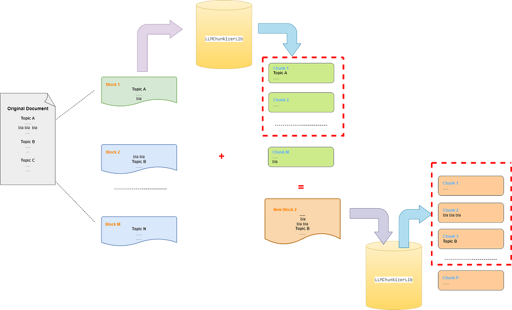
    Process to split first two blocks
    The process of splitting two blocks — Image by the author

    This article explains how to use an LLM (Large Language Model) to perform the chunking of a document based on concept of “idea”.

    I use OpenAI’s gpt-4o model for this example, but the same approach can be applied with any other LLM, such as those from Hugging Face, Mistral, and others.

    Everyone can access this article for free.

    Considerations on Document Chunking

    In cognitive psychology, a chunk represents a “unit of information.”

    This concept can be applied to computing as well: using an LLM, we can analyze a document and produce a set of chunks, typically of variable length, with each chunk expressing a complete “idea.”

    This means that the system divides a document into “pieces of text” such that each expresses a unified concept, without mixing different ideas in the same chunk.

    The goal is to create a knowledge base composed of independent elements that can be related to one another without overlapping different concepts within the same chunk.

    Of course, during analysis and division, there may be multiple chunks expressing the same idea if that idea is repeated in different sections or expressed differently within the same document.

    Getting Started

    The first step is identifying a document that will be part of our knowledge base.

    This is typically a PDF or Word document, read either page by page or by paragraphs and converted into text.

    For simplicity, let’s assume we already have a list of text paragraphs like the following, extracted from Around the World in Eighty Days:

    documents = [
    """On October 2, 1872, Phileas Fogg, an English gentleman, left London for an extraordinary journey.
    He had wagered that he could circumnavigate the globe in just eighty days.
    Fogg was a man of strict habits and a very methodical life; everything was planned down to the smallest detail, and nothing was left to chance.
    He departed London on a train to Dover, then crossed the Channel by ship. His journey took him through many countries,
    including France, India, Japan, and America. At each stop, he encountered various people and faced countless adventures, but his determination never wavered.""",

    """However, time was his enemy, and any delay risked losing the bet. With the help of his faithful servant Passepartout, Fogg had to face
    unexpected obstacles and dangerous situations.""",

    """Yet, each time, his cunning and indomitable spirit guided him to victory, while the world watched in disbelief.""",

    """With one final effort, Fogg and Passepartout reached London just in time to prove that they had completed their journey in less than eighty days.
    This extraordinary adventurer not only won the bet but also discovered that the true treasure was the friendship and experiences he had accumulated along the way."""
    ]

    Let’s also assume we are using an LLM that accepts a limited number of tokens for input and output, which we’ll call input_token_nr and output_token_nr.

    For this example, we’ll set input_token_nr = 300 and output_token_nr = 250.

    This means that for successful splitting, the number of tokens for both the prompt and the document to be analyzed must be less than 300, while the result produced by the LLM must consume no more than 250 tokens.

    Using the tokenizer provided by OpenAI we see that our knowledge base documents is composed of 254 tokens.

    Therefore, analyzing the entire document at once isn’t possible, as even though the input can be processed in a single call, it can’t fit in the output.

    So, as a preparatory step, we need to divide the original document into blocks no larger than 250 tokens.

    These blocks will then be passed to the LLM, which will further split them into chunks.

    To be cautious, let’s set the maximum block size to 200 tokens.

    Generating Blocks

    The process of generating blocks is as follows:

    1. Consider the first paragraph in the knowledge base (KB), determine the number of tokens it requires, and if it’s less than 200, it becomes the first element of the block.
    2. Analyze the size of the next paragraph, and if the combined size with the current block is less than 200 tokens, add it to the block and continue with the remaining paragraphs.
    3. A block reaches its maximum size when attempting to add another paragraph causes the block size to exceed the limit.
    4. Repeat from step one until all paragraphs have been processed.

    The blocks generation process assumes, for simplicity, that each paragraph is smaller than the maximum allowed size (otherwise, the paragraph itself must be split into smaller elements).

    To perform this task, we use the llm_chunkizer.split_document_into_blocks function from the LLMChunkizerLib/chunkizer.py library, which can be found in the following repository — LLMChunkizer.

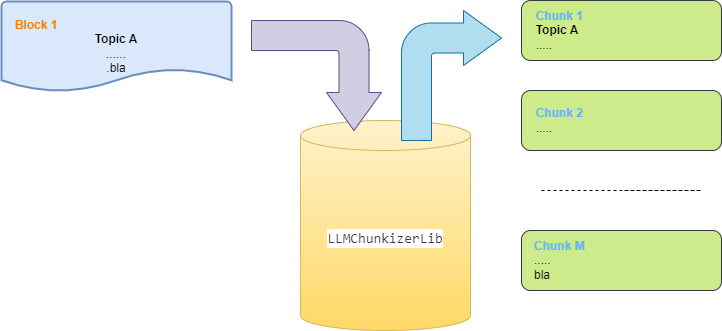
    Visually, the result looks like Figure 1.

    Figure 1 — Split document into blocks of maximum size of 200 tokens — Image by the author

    When generating blocks, the only rule to follow is not to exceed the maximum allowed size.

    No analysis or assumptions are made about the meaning of the text.

    Generating Chunks

    The next step is to split the block into chunks that each express the same idea.

    For this task, we use the llm_chunkizer.chunk_text_with_llm function from the LLMChunkizerLib/chunkizer.py library, also found in the same repository.

    The result can be seen in Figure 2.

    see the process of splitting a block into chunks
    Figure 2 — Split block into chunks — Image by the author

    This process works linearly, allowing the LLM to freely decide how to form the chunks.

    Handling the Overlap Between Two Blocks

    As previously mentioned, during block splitting, only the length limit is considered, with no regard for whether adjacent paragraphs expressing the same idea are split across different blocks.

    This is evident in Figure 1, where the concept “bla bla bla” (representing a unified idea) is split between two adjacent blocks.

    As you can see In Figure 2, the chunkizer processes only one block at a time, meaning the LLM cannot correlate this information with the following block (it doesn’t even know a next block exists), and thus, places it in the last split chunk.

    This problem occurs frequently during ingestion, particularly when importing a long document whose text cannot all fit within a single LLM prompt.

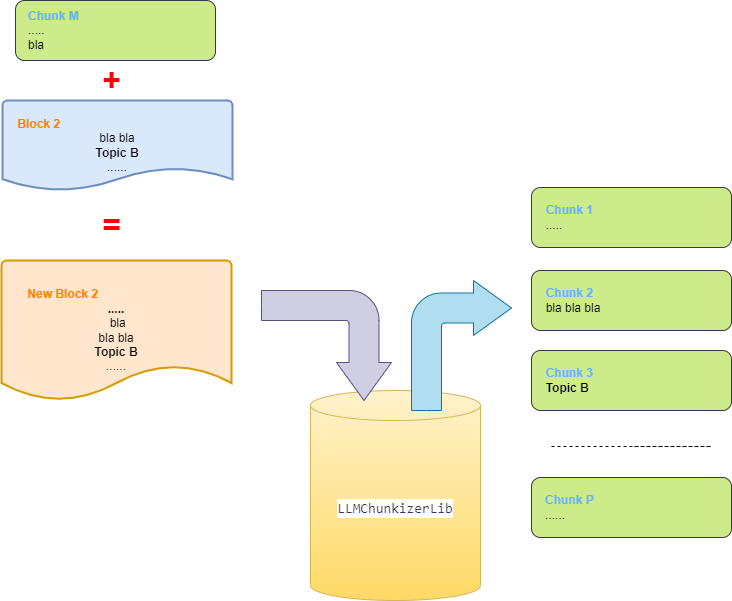
    To address it, llm_chunkizer.chunk_text_with_llm works as shown in Figure 3:

    1. The last chunk (or the last N chunks) produced from the previous block is removed from the “valid” chunks list, and its content is added to the next block to be split.
    2. The New Block2 is passed to the chunking function again.
    See the process to handling the overlap between two blocks
    Figure 3 — Handling the overlap — Image by the author

    As shown in Figure 3, the content of chunk M is split more effectively into two chunks, keeping the concept “bla bla bla” together

    The idea behind this solution is that the last N chunks of the previous block represent independent ideas, not just unrelated paragraphs.

    Therefore, adding them to the new block allows the LLM to generate similar chunks while also creating a new chunk that unites paragraphs that were previously split without regard for their meaning.

    Result of Chunking

    At the end, the system produces the following 6 chunks:

    0: On October 2, 1872, Phileas Fogg, an English gentleman, left London for an extraordinary journey. He had wagered that he could circumnavigate the globe in just eighty days. Fogg was a man of strict habits and a very methodical life; everything was planned down to the smallest detail, and nothing was left to chance.  
    1: He departed London on a train to Dover, then crossed the Channel by ship. His journey took him through many countries, including France, India, Japan, and America. At each stop, he encountered various people and faced countless adventures, but his determination never wavered.
    2: However, time was his enemy, and any delay risked losing the bet. With the help of his faithful servant Passepartout, Fogg had to face unexpected obstacles and dangerous situations.
    3: Yet, each time, his cunning and indomitable spirit guided him to victory, while the world watched in disbelief.
    4: With one final effort, Fogg and Passepartout reached London just in time to prove that they had completed their journey in less than eighty days.
    5: This extraordinary adventurer not only won the bet but also discovered that the true treasure was the friendship and experiences he had accumulated along the way.

    Considerations on Block Size

    Let’s see what happens when the original document is split into larger blocks with a maximum size of 1000 tokens.

    With larger block sizes, the system generates 4 chunks instead of 6.

    This behavior is expected because the LLM could analyzed a larger portion of content at once and was able to use more text to represent a single concept.

    Here are the chunks in this case:

    0: On October 2, 1872, Phileas Fogg, an English gentleman, left London for an extraordinary journey. He had wagered that he could circumnavigate the globe in just eighty days. Fogg was a man of strict habits and a very methodical life; everything was planned down to the smallest detail, and nothing was left to chance.  
    1: He departed London on a train to Dover, then crossed the Channel by ship. His journey took him through many countries, including France, India, Japan, and America. At each stop, he encountered various people and faced countless adventures, but his determination never wavered.
    2: However, time was his enemy, and any delay risked losing the bet. With the help of his faithful servant Passepartout, Fogg had to face unexpected obstacles and dangerous situations. Yet, each time, his cunning and indomitable spirit guided him to victory, while the world watched in disbelief.
    3: With one final effort, Fogg and Passepartout reached London just in time to prove that they had completed their journey in less than eighty days. This extraordinary adventurer not only won the bet but also discovered that the true treasure was the friendship and experiences he had accumulated along the way.

    Conclusions

    It’s important to attempt multiple chunking runs, varying the block size passed to the chunkizer each time.

    After each attempt, the results should be reviewed to determine which approach best fits the desired outcome.

    Coming Up

    In the next article, I will show how to use an LLM to retrieve chunks — LLMRetriever .

    You could find all the code and more example in my repository — LLMChunkizer.

    If you’d like to discuss this further, feel free to connect with me on LinkedIn


    Efficient Document Chunking Using LLMs: Unlocking Knowledge One Block at a Time was originally published in Towards Data Science on Medium, where people are continuing the conversation by highlighting and responding to this story.

    Originally appeared here:
    Efficient Document Chunking Using LLMs: Unlocking Knowledge One Block at a Time

    Go Here to Read this Fast! Efficient Document Chunking Using LLMs: Unlocking Knowledge One Block at a Time

  • Deploy a serverless web application to edit images using Amazon Bedrock

    Deploy a serverless web application to edit images using Amazon Bedrock

    Salman Ahmed

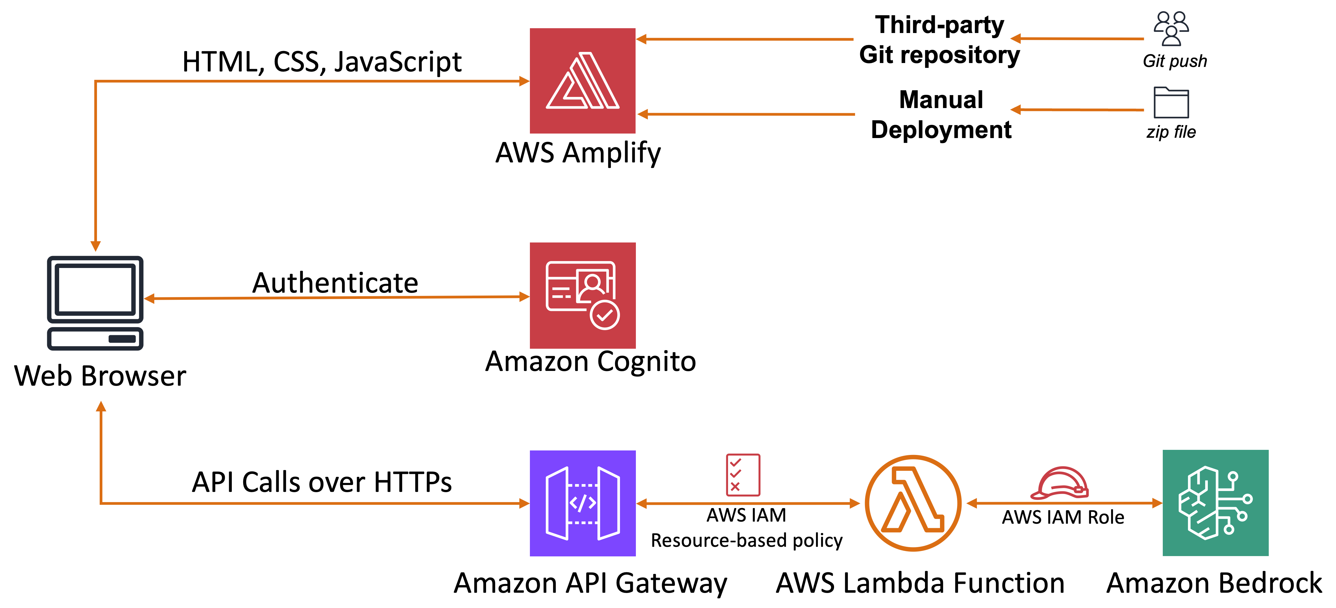
    In this post, we explore a sample solution that you can use to deploy an image editing application by using AWS serverless services and generative AI services. We use Amazon Bedrock and an Amazon Titan FM that allow you to edit images by using prompts.

    Originally appeared here:
    Deploy a serverless web application to edit images using Amazon Bedrock

    Go Here to Read this Fast! Deploy a serverless web application to edit images using Amazon Bedrock

  • Brilliant words, brilliant writing: Using AWS AI chips to quickly deploy Meta LLama 3-powered applications

    Brilliant words, brilliant writing: Using AWS AI chips to quickly deploy Meta LLama 3-powered applications

    Zheng Zhang

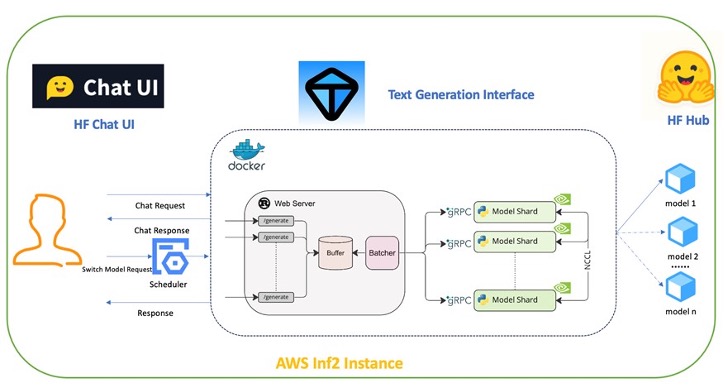
    In this post, we will introduce how to use an Amazon EC2 Inf2 instance to cost-effectively deploy multiple industry-leading LLMs on AWS Inferentia2, a purpose-built AWS AI chip, helping customers to quickly test and open up an API interface to facilitate performance benchmarking and downstream application calls at the same time.

    Originally appeared here:
    Brilliant words, brilliant writing: Using AWS AI chips to quickly deploy Meta LLama 3-powered applications

    Go Here to Read this Fast! Brilliant words, brilliant writing: Using AWS AI chips to quickly deploy Meta LLama 3-powered applications

  • Evaluating Model Retraining Strategies

    Evaluating Model Retraining Strategies

    Reinhard Sellmair

    How data drift and concept drift matter to choose the right retraining strategy?

    (created with Image Creator in Bing)

    Introduction

    Many people in the field of MLOps have probably heard a story like this:

    Company A embarked on an ambitious quest to harness the power of machine learning. It was a journey fraught with challenges, as the team struggled to pinpoint a topic that would not only leverage the prowess of machine learning but also deliver tangible business value. After many brainstorming sessions, they finally settled on a use case that promised to revolutionize their operations. With excitement, they contracted Company B, a reputed expert, to build and deploy a ML model. Following months of rigorous development and testing, the model passed all acceptance criteria, marking a significant milestone for Company A, who looked forward to future opportunities.

    However, as time passed, the model began producing unexpected results, rendering it ineffective for its intended use. Company A reached out to Company B for advice, only to learn that the changed circumstances required building a new model, necessitating an even higher investment as the original.

    What went wrong? Was the model Company B created not as good as expected? Was Company A just unlucky that something unexpected happened?

    Probably the issue was that even the most rigorous testing of a model before deployment does not guarantee that this model will perform well for an unlimited amount of time. The two most important aspects that impact a model’s performance over time are data drift and concept drift.

    Data Drift: Also known as covariate shift, this occurs when the statistical properties of the input data change over time. If an ML model was trained on data from a specific demographic but the demographic characteristics of the input data change, the model’s performance can degrade. Imagine you taught a child multiplication tables until 10. It can quickly give you the correct answers for what is 3 * 7 or 4 * 9. However, one time you ask what is 4 * 13, and although the rules of multiplication did not change it may give you the wrong answer because it did not memorize the solution.

    Concept Drift: This happens when the relationship between the input data and the target variable changes. This can lead to a degradation in model performance as the model’s predictions no longer align with the evolving data patterns. An example here could be spelling reforms. When you were a child, you may have learned to write “co-operate”, however now it is written as “cooperate”. Although you mean the same word, your output of writing that word has changed over time.

    In this article I investigate how different scenarios of data drift and concept drift impact a model’s performance over time. Furthermore, I show what retraining strategies can mitigate performance degradation.

    I focus on evaluating retraining strategies with respect to the model’s prediction performance. In practice more aspects like:

    • Data Availability and Quality: Ensure that sufficient and high-quality data is available for retraining the model.
    • Computational Costs: Evaluate the computational resources required for retraining, including hardware and processing time.
    • Business Impact: Consider the potential impact on business operations and outcomes when choosing a retraining strategy.
    • Regulatory Compliance: Ensure that the retraining strategy complies with any relevant regulations and standards, e.g. anti-discrimination.

    need to be considered to identify a suitable retraining strategy.

    Data Synthetization

    (created with Image Creator in Bing)

    To highlight the differences between data drift and concept drift I synthesized datasets where I controlled to what extent these aspects appear.

    I generated datasets in 100 steps where I changed parameters incrementally to simulate the evolution of the dataset. Each step contains multiple data points and can be interpreted as the amount of data that was collected over an hour, a day or a week. After every step the model was re-evaluated and could be retrained.

    To create the datasets, I first randomly sampled features from a normal distribution where mean µ and standard deviation σ depend on the step number s:

    The data drift of feature xi depends on how much µi and σi are changing with respect to the step number s.

    All features are aggregated as follows:

    Where ci are coefficients that describe the impact of feature xi on X. Concept drift can be controlled by changing these coefficients with respect to s. A random number ε which is not available for model training is added to consider that the features do not contain complete information to predict the target y.

    The target variable y is calculated by inputting X into a non-linear function. By doing this we create a more challenging task for the ML model since there is no linear relation between the features and the target. For the scenarios in this article, I chose a sine function.

    Scenario Analysis

    (created with Image Creator in Bing)

    I created the following scenarios to analyze:

    • Steady State: simulating no data or concept drift — parameters µ, σ, and c were independent of step s
    • Distribution Drift: simulating data drift — parameters µ, σ were linear functions of s, parameters c is independent of s
    • Coefficient Drift: simulating concept drift: parameters µ, σ were independent of s, parameters c are a linear function of s
    • Black Swan: simulating an unexpected and sudden change — parameters µ, σ, and c were independent of step s except for one step when these parameters were changed

    The COVID-19 pandemic serves as a quintessential example of a Black Swan event. A Black Swan is characterized by its extreme rarity and unexpectedness. COVID-19 could not have been predicted to mitigate its effects beforehand. Many deployed ML models suddenly produced unexpected results and had to be retrained after the outbreak.

    For each scenario I used the first 20 steps as training data of the initial model. For the remaining steps I evaluated three retraining strategies:

    • None: No retraining — the model trained on the training data was used for all remaining steps.
    • All Data: All previous data was used to train a new model, e.g. the model evaluated at step 30 was trained on the data from step 0 to 29.
    • Window: A fixed window size was used to select the training data, e.g. for a window size of 10 the training data at step 30 contained step 20 to 29.

    I used a XG Boost regression model and mean squared error (MSE) as evaluation metric.

    Steady State

    Prediction error of steady state scenario

    The diagram above shows the evaluation results of the steady state scenario. As the first 20 steps were used to train the models the evaluation error was much lower than at later steps. The performance of the None and Window retraining strategies remained at a similar level throughout the scenario. The All Data strategy slightly reduced the prediction error at higher step numbers.

    In this case All Data is the best strategy because it profits from an increasing amount of training data while the models of the other strategies were trained on a constant training data size.

    Distribution Drift (Data Drift)

    Prediction error of distribution drift scenario

    When the input data distributions changed, we can clearly see that the prediction error continuously increased if the model was not retrained on the latest data. Retraining on all data or on a data window resulted in very similar performances. The reason for this is that although All Data was using more data, older data was not relevant for predicting the most recent data.

    Coefficient Drift (Concept Drift)

    Prediction error of coefficient drift scenario

    Changing coefficients means that the importance of features changes over time. In this case we can see that the None retraining strategy had drastic increase of the prediction error. Additionally, the results showed that retraining on all data also lead to a continuous increase of prediction error while the Window retraining strategy kept the prediction error on a constant level.

    The reason why the All Data strategy performance also decreased over time was that the training data contained more and more cases where similar inputs resulted in different outputs. Hence, it became more challenging for the model to identify clear patterns to derive decision rules. This was less of a problem for the Window strategy since older data was ignore which allowed the model to “forget” older patterns and focus on most recent cases.

    Black Swan

    Prediction error of black swan event scenario

    The black swan event occurred at step 39, the errors of all models suddenly increased at this point. However, after retraining a new model on the latest data, the errors of the All Data and Window strategy recovered to the previous level. Which is not the case with the None retraining strategy, here the error increased around 3-fold compared to before the black swan event and remained on that level until the end of the scenario.

    In contrast to the previous scenarios, the black swan event contained both: data drift and concept drift. It is remarkable that the All Data and Window strategy recovered in the same way after the black swan event while we found a significant difference between these strategies in the concept drift scenario. Probably the reason for this is that data drift occurred at the same time as concept drift. Hence, patterns that have been learned on older data were not relevant anymore after the black swan event because the input data has shifted.

    An example for this could be that you are a translator and you get requests to translate a language that you haven’t translated before (data drift). At the same time there was a comprehensive spelling reform of this language (concept drift). While translators who translated this language for many years may be struggling with applying the reform it wouldn’t affect you because you even didn’t know the rules before the reform.

    To reproduce this analysis or explore further you can check out my git repository.

    Conclusion

    Identifying, quantifying, and mitigating the impact of data drift and concept drift is a challenging topic. In this article I analyzed simple scenarios to present basic characteristics of these concepts. More comprehensive analyses will undoubtedly provide deeper and more detailed conclusions on this topic.

    Here is what I learned from this project:

    Mitigating concept drift is more challenging than data drift. While data drift could be handled by basic retraining strategies concept drift requires a more careful selection of training data. Ironically, cases where data drift and concept drift occur at the same time may be easier to handle than pure concept drift cases.

    A comprehensive analysis of the training data would be the ideal starting point of finding an appropriate retraining strategy. Thereby, it is essential to partition the training data with respect to the time when it was recorded. To make the most realistic assessment of the model’s performance, the latest data should only be used as test data. To make an initial assessment regarding data drift and concept drift the remaining training data can be split into two equally sized sets with the older data in one set and the newer data in the other. Comparing feature distributions of these sets allows to assess data drift. Training one model on each set and comparing the change of feature importance would allow to make an initial assessment on concept drift.

    No retraining turned out to be the worst option in all scenarios. Furthermore, in cases where model retraining is not taken into consideration it is also more likely that data to evaluate and/or retrain the model is not collected in an automated way. This means that model performance degradation may be unrecognized or only be noticed at a late stage. Once developers become aware that there is a potential issue with the model precious time would be lost until new data is collected that can be used to retrain the model.

    Identifying the perfect retraining strategy at an early stage is very difficult and may be even impossible if there are unexpected changes in the serving data. Hence, I think a reasonable approach is to start with a retraining strategy that performed well on the partitioned training data. This strategy should be reviewed and updated the time when cases occurred where it did not address changes in the optimal way. Continuous model monitoring is essential to quickly notice and react when the model performance decreases.

    If not otherwise stated all images were created by the author.


    Evaluating Model Retraining Strategies was originally published in Towards Data Science on Medium, where people are continuing the conversation by highlighting and responding to this story.

    Originally appeared here:
    Evaluating Model Retraining Strategies

    Go Here to Read this Fast! Evaluating Model Retraining Strategies