Originally appeared here:
Deep Learning vs Data Science: Who Will Win?
Go Here to Read this Fast! Deep Learning vs Data Science: Who Will Win?

Over the past decade we’ve witnessed the power of scaling deep learning models. Larger models, trained on heaps of data, consistently outperform previous methods in language modelling, image generation, playing games, and even protein folding. To understand why scaling works, let’s look at a toy problem.
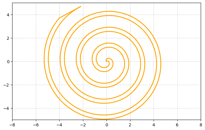
We start with a 1D manifold weaving its way through the 2D plane and forming a spiral:
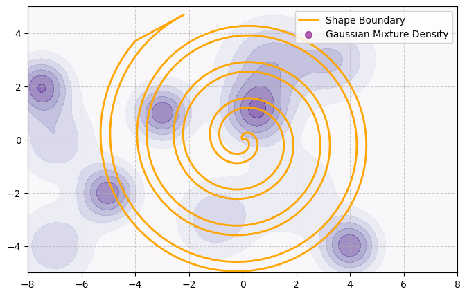
Now we add a heatmap which represents the probability density of sampling a particular 2D point. Notably, this probability density is independent of the shape of the manifold:
Let’s assume that the data on either side of the manifold is always completely separable (i.e. there is no noise). Datapoints on the outside of the manifold are blue and those on the inside are orange. If we draw a sample of N=1000 points it may look like this:
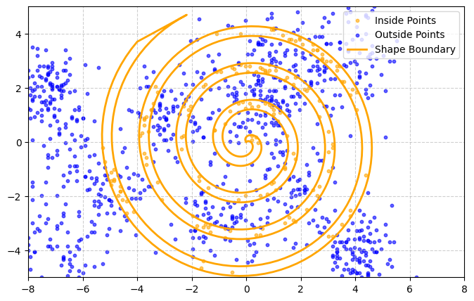
Toy problem: How do we build a model which predicts the colour of a point based on its 2D coordinates?
In the real world we often can’t sample uniformly from all parts of the feature space. For example, in image classification it’s easy to find images of trees in general but less easy to find many examples of specific trees. As a result, it may be harder for a model to learn the difference between species there aren’t many examples of. Similarly, in our toy problem, different parts of the space will become difficult to predict simply because they are harder to sample.
First, we build a simple neural network with 3 layers, running for 1000 epochs. The neural network’s predictions are heavily influenced by the particulars of the sample. As a result, the trained model has difficulty inferring the shape of the manifold just because of sampling sparsity:
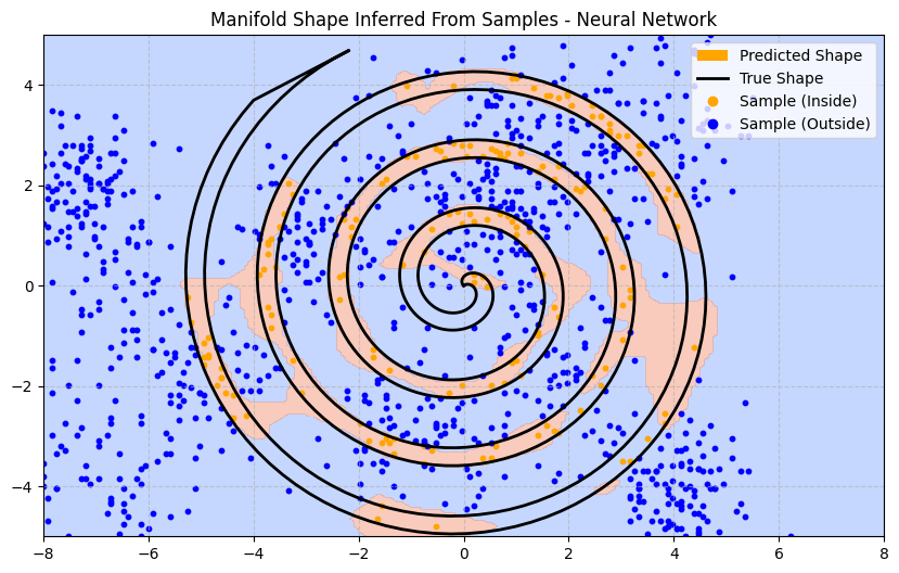
Even knowing that the points are completely separable, there are infinitely many ways to draw a boundary around the sampled points. Based on the sample data, why should any one boundary be considered superior to another?
With regularisation techniques we could encourage the model to produce a smoother boundary rather than curving tightly around predicted points. That helps to an extent but it won’t solve our problem in regions of sparsity.
Since we already know the manifold is a spiral, can we encourage the model to make spiral-like predictions?
We can add what’s called an “inductive prior”: something we put in the model architecture or the training process which contains information about the problem space. In this toy problem we can do some feature engineering and adjust the way we present inputs to the model. Instead of 2D (x, y) coordinates, we transform the input into polar coordinates (r, θ).
Now the neural network can make predictions based on the distance and angle from the origin. This biases the model towards producing decision boundaries which are more curved. Here is how the newly trained model predicts the decision boundary:
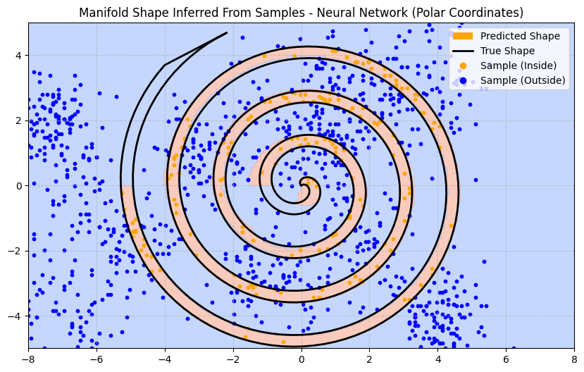
Notice how much better the model performs in parts of the input space where there are no samples. The feature of those missing points remain similar to features of observed points and so the model can predict an effective boundary without seeing additional data.
Obviously, inductive priors are useful.
Most architecture decisions will induce an inductive prior. Let’s try some enhancements and try to think about what kind of inductive prior they introduce:
After making all of these improvements, how much better does our predicted manifold look?
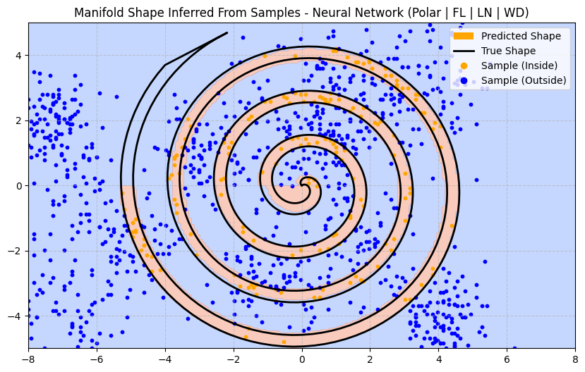
Not much better at all. In fact, it’s introduced an artefact near the centre of the spiral. And it’s still failed to predict anything at the end of the spiral (in the upper-left quadrant) where there is no data. That said, it has managed to capture more of the curve near the origin which is a plus.
Now suppose that another research team has no idea that there’s a hard boundary in the shape of a single continuous spiral. For all they know there could be pockets inside pockets with fuzzy probabilistic boundaries.
However, this team is able to collect a sample of 10,000 instead of 1,000. For their model they just use a k-Nearest Neighbour (kNN) approach with k=5.
Side note: k=5 is a poor inductive prior here. For this problem k=1 is generally better. Challenge: can you figure out why? Add a comment to this article with your answer.
Now, kNN is not a particularly powerful algorithm compared to a neural network. However, even with a bad inductive prior here is how the kNN solution scales with 10x more data:
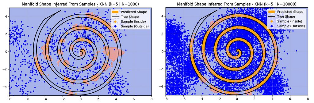
With 10x more data the kNN approach is performing closer to the neural network. In particular it’s better at predicting the shape at the tails of the spiral, although it’s still missing that hard to sample upper-left quadrant. It’s also making some mistakes, often producing a fuzzier border.
What if we added 100x or 1000x more data? Let’s see how both the kNN vs Neural Network approaches compare as we scale the amount of data used:
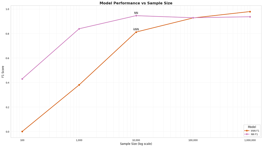
As we increase the size of the training data it largely doesn’t matter which model we use. What’s more, given enough data, the lowly kNN actually starts to perform better than our carefully crafted neural network with well thought out inductive priors.
This is a big lesson. As a field, we still have not thoroughly learned it, as we are continuing to make the same kind of mistakes. To see this, and to effectively resist it, we have to understand the appeal of these mistakes. We have to learn the bitter lesson that building in how we think we think does not work in the long run. The bitter lesson is based on the historical observations that 1) AI researchers have often tried to build knowledge into their agents, 2) this always helps in the short term, and is personally satisfying to the researcher, but 3) in the long run it plateaus and even inhibits further progress, and 4) breakthrough progress eventually arrives by an opposing approach based on scaling computation by search and learning. The eventual success is tinged with bitterness, and often incompletely digested, because it is success over a favored, human-centric approach.
From Rich Sutton’s essay “The Bitter Lesson”
Superior inductive priors are no match for just using more compute to solve the problem. In this case, “more compute” just involves storing a larger sample of data in memory and using kNN to match to the nearest neighbours. We’ve seen this play out with transformer-based Large Language Models (LLMs). They continue to overpower other Natural Language Processing techniques simply by training larger and larger models, with more and more GPUs, on more and more text data.
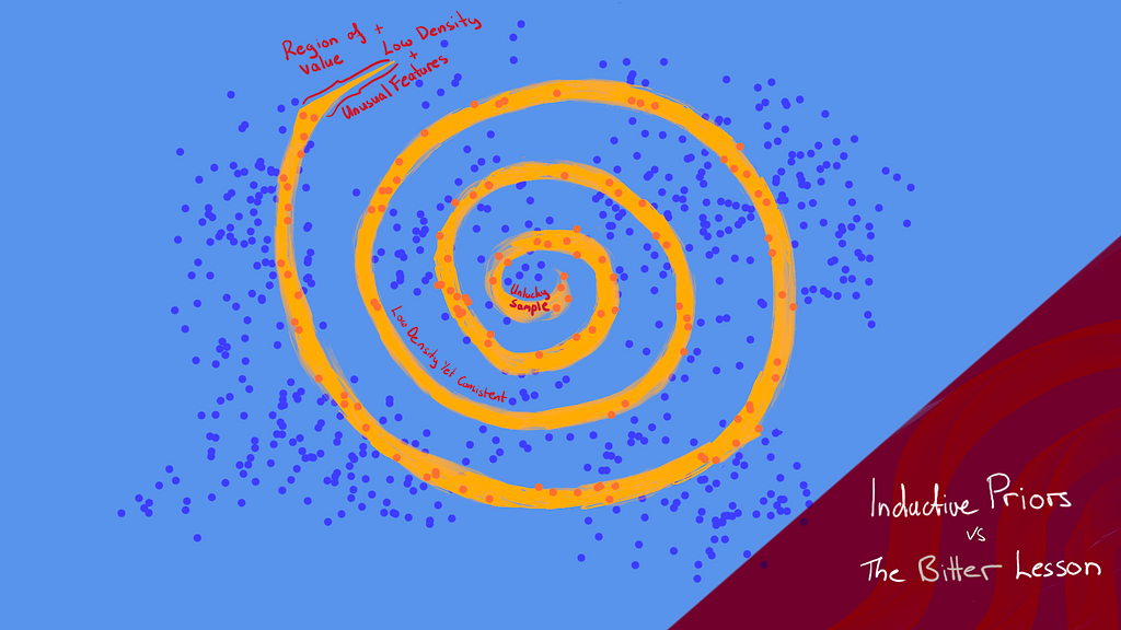
This toy example has a subtle issue we’ve seen pop up with both models: failing to predict that sparse section of the spiral in the upper-left quadrant. This is particularly relevant to Large Language Models, training reasoning capabilities, and our quest towards “Artificial General Intelligence” (AGI). To see what I mean let’s zoom in on that unusual shaped tail in the upper-left.
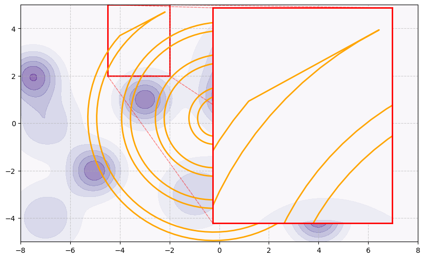
This region has a particularly low sampling density and the boundary is quite different to the rest of the manifold. Suppose this area is something we care a lot about, for example: generating “reasoning” from a Large Language Model (LLM). Not only is such data rare (if randomly sampled) but it is sufficiently different to the rest of the data, which means features from other parts of the space are not useful in making predictions here. Additionally, notice how sharp and specific the boundary is — points sampled near the tip could very easily fall on the outside.
Let’s see how this compares to a simplified view of training an LLM on text-based reasoning:
Of course reasoning is more complex than predicting the tip of this spiral. There are usually multiple ways to get to a correct answer, there may be many correct answers, and sometimes the boundary can be fuzzy. However, we are also not without inductive priors in deep learning architectures, including techniques using reinforcement learning.
In our toy problem there is regularity in the shape of the boundary and so we used an inductive prior to encourage the model to learn that shape. When modelling reasoning, if we could construct a manifold in a higher dimensional space representing concepts and ideas, there would be some regularity to its shape that could be exploited for an inductive prior. If The Bitter Lesson continues to hold then we would assume the search for such an inductive prior is not the path forward. We just need to scale compute. And so far the best way to do that is to collect more data and throw it at larger models.
But surely, I hear you say, transformers were so successful because the attention mechanism introduced a strong inductive prior into language modelling? The paper “Were RNNs all we needed” suggests that a simplified Recurrent Neural Network (RNN) can also perform well if scaled up. It’s not because of an inductive prior. It’s because the paper improved the speed with which we can train an RNN on large amounts of data. And that’s why transformers are so effective — parallelism allowed us to leverage much more compute. It’s an architecture straight from the heart of The Bitter Lesson.
There’s always more data. Synthetic data or reinforcement learning techniques like self-play can generate infinite data. Although without connection to the real world the validity of that data can get fuzzy. That’s why techniques like RLHF have hand crafted data as a base — so that the model of human preferences can be as accurate as possible. Also, given that reasoning is often mathematical, it may be easy to generate such data using automated methods.
Now the question is: given the current inductive priors we have, how much data would it take to train models with true reasoning capability?
If The Bitter Lesson continues to apply the answer is: it doesn’t matter, finding better ways to leverage more compute will continue to give better gains than trying to find superior inductive priors^. This means that the search for ever more powerful AI is firmly in the domain of the companies with the biggest budgets.
And after writing all of this… I still hope that’s not true.
I’m the Lead AI Engineer @ Affinda. Check out our AI Document Automation Case Studies to learn more.
Some of my long reads:
More practical reads:
^ It’s important to note that the essay “The Bitter Lesson” isn’t explicitly about inductive biases vs collecting more data. Throwing more data at bigger models is one way to leverage more compute. And in deep learning that usually means finding better ways to increase parallelism in training. Lately it’s also about leveraging more inference time compute (e.g. o1-preview). There may yet be other ways. The topic is slightly more nuanced than I’ve presented here in this short article.
Why Scaling Works: Inductive Biases vs The Bitter Lesson was originally published in Towards Data Science on Medium, where people are continuing the conversation by highlighting and responding to this story.
Originally appeared here:
Why Scaling Works: Inductive Biases vs The Bitter Lesson
Go Here to Read this Fast! Why Scaling Works: Inductive Biases vs The Bitter Lesson
Game theory is prevalent in real-life scenarios and decision-making
Originally appeared here:
Game Theory, Part 1 — The Prisoner’s Dilemma Problem
Go Here to Read this Fast! Game Theory, Part 1 — The Prisoner’s Dilemma Problem


Exploring the Research on Vector Steering and Coding Up an Implementation
Originally appeared here:
Using Vector Steering to Improve Model Guidance
Go Here to Read this Fast! Using Vector Steering to Improve Model Guidance


A Practical Guide to Applying Probability Concepts with Python in Real-World Contexts
Originally appeared here:
Unleash the Power of Probability to Predict the Future of Your Business
Go Here to Read this Fast! Unleash the Power of Probability to Predict the Future of Your Business


Anyone working with business intelligence, data science, data analysis, or cloud computing will have come across SQL at some point. We can…
Originally appeared here:
SQL and Data Modelling in Action: A Deep Dive into Data Lakehouses
Go Here to Read this Fast! SQL and Data Modelling in Action: A Deep Dive into Data Lakehouses

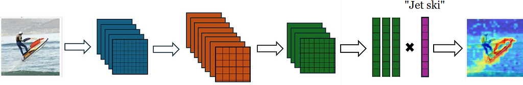
Think of your favorite pre-trained vision encoder. I’m going to assume you’ve chosen some variant of a CNN (Convolutional Neural Network) or a ViT (Visual Transformer). The encoder is a function that maps an image into a d-dimensional vector space. In the process, the image is transformed into a sequence of feature maps:
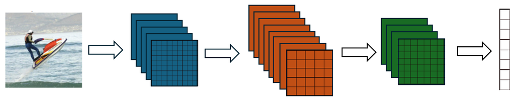
A feature map (w × h × k) can be thought of as a collected 2D array of k-dimensional patch embeddings, or, equivalently, a coarse image (w × h) with k channels f₁, … fₖ. Both CNNs and ViTs, in their respective ways, are in the business of transforming an input image into a sequence of feature maps.
How can we see what a vision encoder sees as an image make its way through its layers? Zero-shot localization methods are designed to generate human-interpretable visualizations from an encoder’s feature maps. These visualizations, which can look like heatmaps or coarse segmentation masks, discriminate between semantically related regions in the input image. The term “zero-shot” refers to the fact that the model has not explicitly been trained on mask annotations for the semantic categories of interest. A vision encoder like CLIP, for instance, has only been trained on image-level text captions.
In this article, we begin with an overview of some early techniques for generating interpretable heatmaps from supervised CNN classifiers, with no additional training required. We then explore the challenges around achieving zero-shot localization with CLIP-style encoders. Finally, we touch on the key ideas behind GEM (Grounding Everything Module) [1], a recently proposed approach to training-free, open-vocabulary localization for the CLIP ViT.
Let’s build some intuition around the concept of localization by considering a simple vision encoder trained for image classification in a supervised way. Assume the CNN uses:
The logit for a given class c can then be written as:

where Wᵢ(c) denotes the (scalar) weight of feature channel i on logit c, and Zᵢ is a normalizing constant for the average pooling.
The key observation behind Class Activation Maps [2] is that the above summation can be re-written as:

In other words, the logit can be expressed as a weighted average of the final feature channels which is then averaged across the width and height dimensions.
It turns out that the weighted average of the fᵢ ’s alone gives an interpretable heatmap for class c, where larger values match regions in the image that are more semantically related to the class. This coarse heatmap, which can be up-sampled to match the dimensions of the input image, is called a Class Activation Map (CAM):

Intuitively, each fᵢ is already a heatmap for some latent concept (or “feature”) in the image — though these do not necessarily discriminate between human-interpretable classes in any obvious way. The weight Wᵢ(c) captures the importance of fᵢ in predicting class c. The weighted average thus highlights which image features are most relevant to class c. In this way, we can achieve discriminative localization of the class c without any additional training.
The challenge with class activation maps is that they are only meaningful under certain assumptions about the architecture of the CNN encoder. Grad-CAM [3], proposed in 2019, is an elegant generalization of class activation maps that can be applied to any CNN architecture, as long as the mapping of the final feature map channels f₁, …, fₖ to the logit vector is differentiable.
As in the CAM approach, Grad-CAM computes a weighted sum of feature channels fᵢ to generate an interpretable heatmap for a class c, but the weight for each fᵢ is computed as:
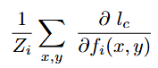
Grad-CAM generalizes the idea of weighing each fᵢ proportionally to its importance for predicting the logit for class c, as measured by the average-pooled gradients of the logit with respect to elements fᵢ(x, y). Indeed, it can be shown that computing the Grad-CAM weights for a CNN that obeys assumptions 1–2 from the previous section results in the same expression for CAM(c) we saw earlier, up to a normalizing constant (see [3] for a proof).
Grad-CAM also goes a step further by applying ReLU on top of the weighted average of the feature channels fᵢ. The idea is to only visualize features which would strengthen the confidence in the prediction of class c should their intensity be increased. Once again, the output can then be up-sampled to give a heatmap that matches the dimensions of the original input image.
Do these early approaches generalize to CLIP-style encoders? There are two additional complexities to consider with CLIP:
That said, if we could somehow achieve zero-shot localization with CLIP, then we would unlock the ability to perform zero-shot, open-vocabulary localization: in other words, we could generate heatmaps for arbitrary semantic classes. This is the motivation for developing localization methods for CLIP-style encoders.
Let’s first attempt some seemingly reasonable approaches to this problem given our knowledge of localization using supervised CNNs.
For a given input image, the logit for a class c can be computed as the cosine similarity between the CLIP text embedding of the class name and the CLIP image embedding. The gradient of this logit with respect to the image encoder’s final feature map is tractable. Hence, one possible approach would be to directly apply Grad-CAM — and this could work regardless of whether the image encoder is a ViT or a CNN.

Another seemingly reasonable approach might be to consider alignment between image patch embeddings and class text embeddings. Recall that CLIP is trained to maximize alignment between an image-level embedding (specifically, the CLS token embedding) and a corresponding text embedding. Is it possible that this objective implicitly aligns a patch in embedding space more closely to text that is more relevant to it? If this were the case, we could expect to generate a discriminative heatmap for a given class by simply visualizing the similarity between its text embedding and each patch embedding:
Interestingly, not only do both these approaches fail, but the resulting heatmaps turn out to be the opposite of what we would expect. This phenomenon, first described in the paper “Exploring Visual Explanations for Contrastive Language-Image Pre-training” [4], has been observed consistently across different CLIP architectures and across different classes. To see examples of these “opposite visualization” with both patch-text similarity maps and Grad-CAM, take a look at page 19 in the pre-print “A Closer Look at the Explainability of Contrastive Language-Image Pre-training” [5]. As of today, there is no single, complete explanation for this phenomenon, though some partial hypotheses have been proposed.
One such hypothesis is detailed in the aforementioned paper [5]. This work restricts its scope to the ViT architecture and examines attention maps in the final self-attention block of the CLIP ViT. For a given input image and text class, these attention maps (w × h) are computed as follows:
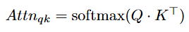
You might expect the anchor patch to be attending mostly to other patches in the image that are semantically related to the class of interest. Instead, these query-key attention maps reveal that anchor patches consistently attend to unrelated patches just as much. As a result, query-key attention maps are blotchy and difficult to interpret (see the paper [5] for some examples). This, the authors suggest, could explain the noisy patch-text similarity maps observed in the CLIP ViT.
On the other hand, the authors find that value-value attention maps are more promising. Empirically, they show that value-value attention weights are larger exclusively for patches near the anchor that are semantically related to it. Value-value attention maps are not complete discriminative heatmaps, but they are a more promising starting point.
Hopefully, you can now see why training-free localization is not as straightforward for CLIP as it was for supervised CNNs — and it is not well-understood why. That said, a recent localization method for the CLIP ViT called the Grounding Everything Module (GEM) [1], proposed in 2024, achieves remarkable success. GEM is essentially a training-free method to correct the noisy query-key attention maps we saw in the previous section. In doing so, the GEM-modified CLIP encoder can be used for zero-shot, open-vocabulary localization. Let’s explore how it works.
The main idea behind GEM is called self-self attention, which is a generalization of the concept of value-value attention.
Given queries Q, keys K and values V, the output of a self-self attention block is computed by applying query-query, key-key, and value-value attention iteratively for t = 0, …, n:
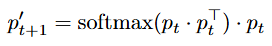

where p₀ ∈ {Q, K, V} and n, the number of iterations, is a hyperparameter. This iterative process can be thought of as clustering the initial tokens p₀ based on dot-product similarity. By the end of this process, the resulting tokens pₙ is a set of cluster “centers” for the initial tokens p₀.
The resulting self-self attention weights are then ensembled to produce the output of the self-self attention block:

where:
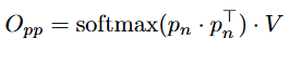
This is in contrast to a traditional query-key attention block, whose output is computed simply as:

Now consider our method for generating value-value attention maps in the previous section, where we first chose an anchor patch based on similarity to a class text embedding, then computed value-value attention map. GEM can be thought of as the reverse of this process, where:
This set of logits can then be reshaped to produce a discriminative heatmap for the chosen class, which can take the form of any arbitrary text! Below are some examples of GEM heatmaps for various class prompts (red indicates higher similarity to the class prompt):

Discriminative localization can transform an image-level encoder into a model that can be used for semantic segmentation, without the need for notoriously expensive mask annotations. Moreover, training-free localization is a powerful approach to making vision encoders more explainable, allowing us to see what they see.
For supervised vision models, zero-shot localization began with class activation maps, a technique for a specific kind of CNN architecture. Later, a generalization of this approach, applicable to any supervised CNN architecture, was proposed. When it comes to CLIP-style encoders, however, training-free localization is less straightforward: the phenomenon of opposite visualizations remains largely unexplained and exists across different CLIP encoder architectures. As of today, some localization techniques for the CLIP ViT such as GEM have proven successful. Is there a more generalized approach waiting to be discovered?
Zero-Shot Localization with CLIP-Style Encoders was originally published in Towards Data Science on Medium, where people are continuing the conversation by highlighting and responding to this story.
Originally appeared here:
Zero-Shot Localization with CLIP-Style Encoders
Go Here to Read this Fast! Zero-Shot Localization with CLIP-Style Encoders

We are in a golden age of AI, with cutting-edge models disrupting industries and poised to transform life as we know it. Powering these advancements are increasingly powerful AI accelerators, such as NVIDIA H100 GPUs, Google Cloud TPUs, AWS’s Trainium and Inferentia chips, and more. With the growing number of options comes the challenge of selecting the most optimal platform for our machine learning (ML) workloads — a crucial decision considering the high costs associated with AI computation. Importantly, a comprehensive assessment of each option necessitates ensuring that we are maximizing its utilization to fully leverage its capabilities.
In this post, we will review several techniques for optimizing an ML workload on AWS’s custom-built AI chips using the AWS Neuron SDK. This continues our ongoing series of posts focused on ML model performance analysis and optimization across various platforms and environments (e.g., see here and here). While our primary focus will be on an ML training workload and AWS Inferentia2, the techniques discussed are also applicable to AWS Trainium. (Recall that although AWS Inferentia is primarily designed as an AI inference chip, we have previously demonstrated its effectiveness in training tasks as well.)
Generally speaking, performance optimization is an iterative process that includes a performance analysis step to appropriately identify performance bottlenecks and resource under-utilization (e.g., see here). However, since the techniques we will discuss are general purpose (i.e., they are potentially applicable to any model, regardless of their performance profile), we defer the discussion on performance analysis with the Neuron SDK to a future post.
The code we will share is intended for demonstrative purposes only — we make no claims regarding its accuracy, optimality, or robustness. Please do not view this post as a substitute for the official Neuron SDK documentation. Please do not interpret our mention of any platforms, libraries, or optimization techniques as an endorsement for their use. The best options for you will depend greatly on the specifics of your use-case and will require your own in-depth investigation and analysis.
The experiments described below were run on an Amazon EC2 inf2.xlarge instance (containing two Neuron cores and four vCPUs). We used the most recent version of the Deep Learning AMI for Neuron available at the time of this writing, “Deep Learning AMI Neuron (Ubuntu 22.04) 20240927”, with AWS Neuron 2.20 and PyTorch 2.1. See the SDK documentation for more details on setup and installation. Keep in mind that the Neuron SDK is under active development and that the APIs we refer to, as well as the runtime measurements we report, may become outdated by the time you read this. Please be sure to stay up-to-date with the latest SDK and documentation available.
To facilitate our discussion, we introduce the following simple Vision Transformer (ViT)-backed classification model (based on timm version 1.0.10):
from torch.utils.data import Dataset
import time, os
import torch
import torch_xla.core.xla_model as xm
import torch_xla.distributed.parallel_loader as pl
from timm.models.vision_transformer import VisionTransformer

# use random data
class FakeDataset(Dataset):
  def __len__(self):
    return 1000000

  def __getitem__(self, index):
    rand_image = torch.randn([3, 224, 224], dtype=torch.float32)
    label = torch.tensor(data=index % 1000, dtype=torch.int64)
    return rand_image, label

def train(batch_size=16, num_workers=0):
  # Initialize XLA process group for torchrun
  import torch_xla.distributed.xla_backend
  torch.distributed.init_process_group('xla')

  # multi-processing: ensure each worker has same initial weights
  torch.manual_seed(0)
  dataset = FakeDataset()
  model = VisionTransformer()

  # load model to XLA device
  device = xm.xla_device()
  model = model.to(device)
  optimizer = torch.optim.Adam(model.parameters())
  data_loader = torch.utils.data.DataLoader(dataset,
                                            batch_size=batch_size,
                                            num_workers=num_workers)

  data_loader = pl.MpDeviceLoader(data_loader, device)
  loss_function = torch.nn.CrossEntropyLoss()
  summ = 0
  count = 0
  t0 = time.perf_counter()

  for step, (inputs, targets) in enumerate(data_loader, start=1):
    optimizer.zero_grad()
    outputs = model(inputs)
    loss = loss_function(outputs, targets)
    loss.backward()
    xm.optimizer_step(optimizer)
    batch_time = time.perf_counter() - t0
    if step > 10:  # skip first steps
      summ += batch_time
      count += 1
    t0 = time.perf_counter()
    if step > 500:
      break
  print(f'average step time: {summ/count}')

if __name__ == '__main__':
  train()

# Initialization command:
# torchrun --nproc_per_node=2 train.py
Running our baseline model on the two cores of our AWS Inferentia instance, results in a training speed of 251.98 samples per second.
In the next sections, we will iteratively apply a number of potential optimization techniques and assess their impact on step time performance. While we won’t go into the full details of each method, we will provide references for further reading (e.g., here). Importantly, the list we will present is not all-inclusive — there are many techniques beyond what we will cover. We will organize the methods into three categories: PyTorch optimizations, OpenXLA optimizations, and Neuron-specific optimizations. However, the order of presentation is not binding. In fact, some of the techniques are interdependent — for example, applying the mixed precision optimization may free up enough device memory to enable increasing the batch size.
In previous posts (e.g., here) we have covered the topic of PyTorch model performance analysis and optimization on GPU, extensively. Many of the techniques we discussed are relevant to other AI accelerators. In this section we will revisit few of these techniques and apply them to AWS Inferentia.
In multi process data loading the input data is prepared in one or more dedicated CPU processes rather than in the same process that runs the training step. This allows for overlapping the data loading and training which can increase system utilization and lead to a significant speed-up. The number of processes is controlled by the num_workers parameter of the PyTorch DataLoader. In the following block we run our script with num_workers set to one:
train(num_workers=1)
This change results in a training speed of 253.56 samples per second for a boost of less than 1%.
Another important hyperparameter that can influence training speed is the training batch size. Often, we have found that increasing the batch size improves system utilization and results in better performance. However, the effects can vary based on the model and platform. In the case of our toy model on AWS Inferentia, we find that running with a batch size of 8 samples per neuron core results in a speed of 265.68 samples per second — roughly 5% faster than a batch size of 16 samples per core.
train(batch_size=8, num_workers=1)
Another common method for boosting performance is to use lower precision floats such as the 16-bit BFloat16. Importantly, some model components might not be compatible with reduced precision floats. PyTorch’s Automatic Mixed Precision (AMP) mode attempts to match the most appropriate floating point type to each model operation automatically. Although, the Neuron compiler offers different options for employing mixed precision, it also supports the option of using PyTorch AMP. In the code block below we include the modifications required to use PyTorch AMP.
def train(batch_size=16, num_workers=0):
  # Initialize XLA process group for torchrun
  import torch_xla.distributed.xla_backend
  torch.distributed.init_process_group('xla')

  # multi-processing: ensure each worker has same initial weights
  torch.manual_seed(0)
  dataset = FakeDataset()
  model = VisionTransformer()

  # load model to XLA device
  device = xm.xla_device()
  model = model.to(device)
  optimizer = torch.optim.Adam(model.parameters())
  data_loader = torch.utils.data.DataLoader(dataset,
                                            batch_size=batch_size,
                                            num_workers=num_workers)

  data_loader = pl.MpDeviceLoader(data_loader, device)
  loss_function = torch.nn.CrossEntropyLoss()
  summ = 0
  count = 0
  t0 = time.perf_counter()

  for step, (inputs, targets) in enumerate(data_loader, start=1):
    optimizer.zero_grad()

    # use PyTorch AMP
    with torch.autocast(dtype=torch.bfloat16, device_type='cuda'):
      outputs = model(inputs)
      loss = loss_function(outputs, targets)
    loss.backward()
    xm.optimizer_step(optimizer)
    batch_time = time.perf_counter() - t0
    if step > 10:  # skip first steps
      summ += batch_time
      count += 1
    t0 = time.perf_counter()
    if step > 500:
      break
  print(f'average step time: {summ/count}')

if __name__ == '__main__':
  # disable neuron compilar casting
  os.environ["NEURON_CC_FLAGS"] = "--auto-cast=none"
  torch.cuda.is_bf16_supported = lambda: True
  train(batch_size=8, num_workers=1)
The resultant training speed is 196.64 samples per second, about 26% lower than the default mixed precision setting of the Neuron compiler. It’s important to note that while this post focuses on performance, in real-world scenarios, we would also need to evaluate the effect of the mixed precision policy we choose on model accuracy.
As discussed in a previous post, Neuron Cores are treated as XLA devices and the torch-neuronx Python package implements the PyTorch/XLA API. Consequently, any optimization opportunities provided by the OpenXLA framework, and specifically those offered by the PyTorch/XLA API, can be leveraged on AWS Inferentia and Trainium. In this section we consider a few of these opportunities.
OpenXLA supports the option of casting all floats to BFloat16 via the XLA_USE_BF16 environment variable, as shown in the code block below:
if __name__ == '__main__':
  os.environ['XLA_USE_BF16'] = '1'
  train(batch_size=8, num_workers=1)
The resultant training speed is 394.51 samples per second, nearly 50% faster than the speed of the default mixed precision option.
The PyTorch/XLA MpDeviceLoader and its internal ParallelLoader, which are responsible for loading input data on to the accelerator, include a number of parameters for controlling the transfer of data from the host to the device. In the code block below we tune batches_per_execution setting which determines the number of batches copied to the device for each execution cycle of the ParallelLoader. By increasing this setting, we aim to reduce the overhead of the host-to-device communication:
data_loader = torch.utils.data.DataLoader(dataset,
                                          batch_size=batch_size,
                                          num_workers=num_workers
                                          )
data_loader = pl.MpDeviceLoader(data_loader,
                                device, batches_per_execution=10)
As a result of this optimization, the training speed increased to 1,027.39 samples per second, representing an additional 260% speed-up.
In previous posts (e.g., here), we have demonstrated the potential performance gains from using PyTorch’s graph compilation offering. Although OpenXLA includes its own graph creation and Just-In-Time (JIT) compilation mechanisms, torch.compile can provide additional acceleration by eliminating the need for tracing the model operations at every step. The following code snippet demonstrates the use of the dedicated openxla backend for compiling the model:
model = model.to(device)
model = torch.compile(backend='openxla')
Although torch.compile is currently not yet supported by the Neuron SDK, we include its mention in anticipation of its future release.
In this section we consider some of the optimization opportunities offered by the AWS Neuron SDK and, more specifically, by the Neuron compiler.
The Neuron SDK supports a variety of mixed precision settings. In the code block below we program the compiler to cast all floats to BFloat16 via the NEURON_CC_FLAGS environment variable.
if __name__ == '__main__':
  os.environ["NEURON_CC_FLAGS"] = "--auto-cast all --auto-cast-type bf16"
  train(batch_size=8, num_workers=1)
This results (unsurprisingly) in a similar training speed to the OpenXLA BFloat16 experiment described above.
One of the unique features of NeuronCoreV2 is its support of the eight-bit floating point type, fp8_e4m3. The code block below demonstrates how to configure the Neuron compiler to automatically cast all floating-point operations to FP8:
if __name__ == '__main__':
 os.environ["NEURON_CC_FLAGS"] = "--auto-cast all --auto-cast-type fp8_e4m3"
 train(batch_size=8, num_workers=1)
While FP8 can accelerate training in some cases, maintaining stable convergence can be more challenging than when using BFloat16 due its reduced precision and dynamic range. Please see our previous post for more on the potential benefits and challenges of FP8 training.
In the case of our model, using FP8 actually harms runtime performance compared to BFloat16, reducing the training speed to 940.36 samples per second.
The Neuron compiler includes a number of controls for optimizing the runtime performance of the compiled graph. Two key settings are model-type and opt-level. The model-type setting applies optimizations tailored to specific model architectures, such as transformers, while the opt-level setting allows for balancing compilation time against runtime performance. In the code block below, we program the model-type setting to tranformer and the opt-level setting to the highest performance option. We further specify the target runtime device, inf2, to ensure that the model is optimized for the target device.
if __name__ == '__main__':
  os.environ['XLA_USE_BF16'] = '1'
  os.environ["NEURON_CC_FLAGS"] = "--model-type transformer "
                                  "--optlevel 3"
                                  " --target inf2"
  train(batch_size=8, num_workers=1)
The above configuration resulted in a training speed of 1093.25 samples per second, amounting to a modest 6% improvement.
We summarize the results of our experiments in the table below. Keep in mind that the effect of each of the optimization methods we discussed will depend greatly on the model and the runtime environment.
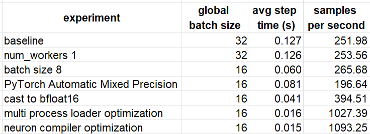
The techniques we employed resulted in a 435% performance boost compared to our baseline experiment. It is likely that additional acceleration could be achieved by revisiting and fine-tuning some of the methods we discussed, or by applying other optimization techniques not covered in this post.
Our goal has been demonstrate some of the available optimization strategies and demonstrate their potential impact on runtime performance. However, in a real-world scenario, we would need to assess the manner in which each of these optimizations impact our model convergence. In some cases, adjustments to the model configuration may be necessary to ensure optimal performance without sacrificing accuracy. Additionally, using a performance profiler to identify bottlenecks and measure system resource utilization is essential for guiding and informing our optimization activities.
Nowadays, we are fortunate to have a wide variety of systems on which to run our ML workloads. No matter which platform we choose, our goal is to maximize its capabilities. In this post, we focused on AWS Inferentia and reviewed several techniques for accelerating ML workloads running on it. Be sure to check out our other posts for more optimization strategies across various AI accelerators.
AI Model Optimization on AWS Inferentia and Trainium was originally published in Towards Data Science on Medium, where people are continuing the conversation by highlighting and responding to this story.
Originally appeared here:
AI Model Optimization on AWS Inferentia and Trainium
Go Here to Read this Fast! AI Model Optimization on AWS Inferentia and Trainium
To state the obvious, data science has evolved into one of the most sought-after skill sets in the market over the past decade. Traditional corporations, technology companies, consulting firms, start-up businesses — you name it — are continually hiring data science professionals. High demand and a relatively short supply of experienced experts in this space make this a very lucrative career opportunity. To break into and be successful in this area, you need a deep understanding of not just the available algorithms and packages but also develop an intuition around which methods lend themselves to which use cases. Plus you’ll need to learn how to translate a real-world problem to a data science framework. In this post, I’ll talk about how beginners can build a fundamental and deep understanding of this space to initiate a career in this area.

Given the plethora of resources available to learners, it can be confusing as to what to pick as a learning mechanism. While it would depend on your individual situation and objective, you may want to consider a few criteria when selecting a learning resource:
· Content: typically, a robust resource will cover supervised learning (e.g. linear regression, logistic regression, decision trees, ensemble methods), unsupervised learning (e.g. clustering, PCA), as well as basics around statistics and probability. Many programs have focused modules on advanced methods including Deep Learning, Computer Vision, Natural Language Processing, and Generative AI. Some programs even offer free previews of the course contents, learning videos, and coding projects to help learners make a decision. While it may be challenging to find a program that includes every topic in detail, your purpose for pivoting into the data science domain should dictate the choice of the coursework.
· Audience: “Who will benefit from the coursework?” is a key question to help with the determination of a program. If you are a beginner, intermediate level courses may prove to be a barrier to learning. On the flip side, very basic concepts may be less useful for learners who already have some background in analytical methods.
· Time commitment: depending on your individual situation and preferences, this consideration may narrow the options you may have. For instance, if you are a working professional, you may not be able to spend beyond a few hours a week. Many online programs offer flexible timings with an expected 5–7 hours of work per week targeted at part-time learners. Overall time spent in a program also determines how much skill development occurs. While advanced programs at universities (e.g. master’s in data science) may serve to develop deeper expertise over 18–24 months and may require several hours of dedicated effort during a week, shorter courses over 4–6 weeks may not be helpful in developing the necessary skills to kickstart a new career.
· Learner experience: you may find user reviews on the program page or at other locations online. These can be helpful in getting a feel for the quality of course content and teaching, especially if there’s a sizeable number of ratings as well as comments. Further, the reach of the program is indicated by the number of learners that are either currently enrolled and/or those who have completed it. One could argue that verifying the validity of reviews and number of learners may be challenging. Even so, these can serve as triangulation points, given other information, for looking at a program holistically.
· Cost: program fees can be an important factor in selection. Programs can range from being free of charge to running into thousands of dollars.
· Career resources: oftentimes, programs offer support for a new job search and career switch, including interview prep, resume reviews, and networking with domain experts in industry. While this may not be a primary consideration regarding choice of a program, these can help get a foot in the door as you start on the career change journey.

While there are several online resources you can use to gain knowledge of specific topics, I would recommend for beginners to consider a structured pathway that provides a comprehensive view of the data science area. Based on my experience, I would recommend choosing from three types of programs, at least initially (one can always supplement the learning with additional material on individual topics):
· Specialization or Professional Certificate
· MicroMasters/Nanodegrees
· Bootcamps
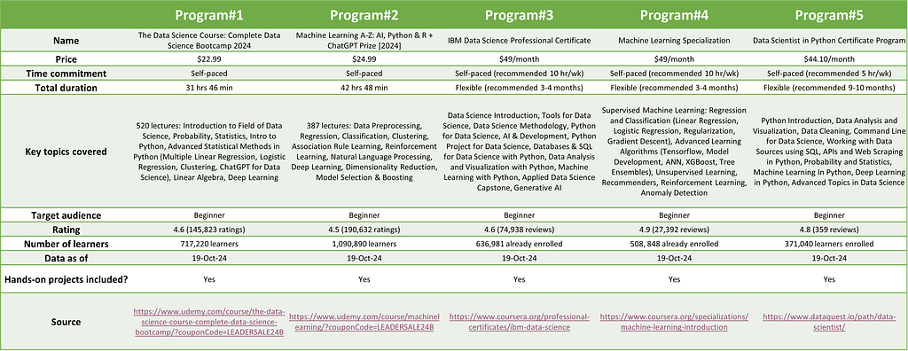
Typically, these programs spread over several months. I have found these to offer a balance between single/short courses that may not be sufficient to develop the required acumen in data science, and formal education that may take more than a year. EdTech companies regularly offer these programs, oftentimes, in collaboration with highly regarded universities. A side-by-side comparison across the selection criteria can be helpful in deciding on a path forward — Figure 1 shows an example comparison of specializations and professional certificates. The courses listed here are only a small sample of the variety of programs online and are by no means exhaustive. Furthermore, the details presented for each program are from a particular point in time and may change.
While it is recommended to select and start with a single program, sometimes it may take multiple courses to feel comfortable with the subject. In my own case, I started with Andrew Ng’s Machine Learning course. It covered the fundamentals in good detail but as the course had exercises in Matlab/Octave at that time, I decided to do another course from IBM to learn Python along with AI/ML. Based on my personal learning preference, I felt the need for a more formal mechanism of instruction and decided to go with a Post Graduate Program in AI/ML from the University of Texas at Austin in collaboration with Great Learning. This provided me with more structure as I had theory to learn from video modules taking up to 5–7 hours per week, take weekly quizzes, attend an online mentor-led group interactive session for a couple of hours every weekend, and code submissions every few weeks. While the theory and quizzes helped me gain an understanding of the concepts, the hands-on code development was really my key to internalizing the learning. This exercise gave me fundamental insights on how to set up the problem, clean and analyze raw data, determine which algorithm to apply, refine the solution, and explain the results.

It is important to make an informed decision when embarking on a skill-building journey. As a beginner, it may be prudent to consider a more structured learning pathway, and then deep dive into specific areas once you have a fair understanding of the basics. Spending time upfront in researching and benchmarking programs can also help learners understand the key and in-demand topics within the data science realm.
Thanks for reading. Hope you found it useful. Feel free to send me your comments to [email protected]. Let’s connect on LinkedIn
How to Get Started on Your Data Science Career Journey was originally published in Towards Data Science on Medium, where people are continuing the conversation by highlighting and responding to this story.
Originally appeared here:
How to Get Started on Your Data Science Career Journey
Go Here to Read this Fast! How to Get Started on Your Data Science Career Journey