In this post, we explore the best practices and lessons learned for fine-tuning Anthropic’s Claude 3 Haiku on Amazon Bedrock. We discuss the important components of fine-tuning, including use case definition, data preparation, model customization, and performance evaluation.
In this post we continue our exploration of the opportunities for runtime optimization of machine learning (ML) workloads through custom operator development. This time, we focus on the tools provided by the AWS Neuron SDK for developing and running new kernels on AWS Trainium and AWS Inferentia. With the rapid development of the low-level model components (e.g., attention layers) driving the AI revolution, the programmability of the accelerators used for training and running ML models is crucial. Dedicated AI chips, in particular, must offer a worthy alternative to the widely used and highly impactful general-purpose GPU (GPGPU) development frameworks, such as CUDA and Triton.
In previous posts (e.g., here and here) we explored the opportunity for building and running ML models on AWS’s custom-built AI chips using the the dedicated AWS Neuron SDK. In its most recent release of the SDK (version 2.20.0), AWS introduced the Neuron Kernel Interface (NKI) for developing custom kernels for NeuronCore-v2, the underlying accelerator powering both Trainium and Inferentia2. The NKI interface joins another API that enables NeuronCore-v2 programmability, Neuron Custom C++ Operators. In this post we will explore both opportunities and demonstrate them in action.
Disclaimers
Importantly, this post should not be viewed as a substitute for the official AWS Neuron SDK documentation. At the time of this writing the Neuron SDK APIs for custom kernel development is in Beta, and may change by the time you read this. The examples we share are intended for demonstrative purposes, only. We make no claims as to their optimality, robustness, durability, or accuracy. Please do not view our mention of any platforms, tools, APIs, etc., as an endorsement for their use. The best choices for any project depend on the specifics of the use-case at hand and warrant appropriate investigation and analysis.
Developing Custom Kernels for Neuron Cores
Although the list of ML models supported by the Neuron SDK is continuously growing, some operations remain either unsupported or implemented suboptimally. By exposing APIs for Neuron kernel customization, the SDK empowers developers to create and/or optimize the low-level operations that they need, greatly increasing the opportunity for running ML workloads on Trainium and Inferentia.
As discussed in our previous posts in this series, fully leveraging the power of these AI chips requires a detailed understanding their low-level architecture.
The Neuron Core Architecture
The NKI documentation includes a dedicated section on the architecture design of NeuronCore-v2 and its implications on custom operator development. Importantly, there are many differences between Neuron cores and their AI accelerator counterparts (e.g., GPUs and TPUs). Optimizing for Neuron cores requires a unique set of strategies and skills.
Similar to other dedicated AI chips, NeuronCore-v2 includes several internal acceleration engines, each of which specializes in performing certain types of computations. The engines can be run asynchronously and in parallel. The Neuron Compiler is responsible for transforming ML models into low-level operations and optimizing the choice of compute engine for each one.
The Tensor engine specializes in matrix multiplication. The Vector and Scalar engines both operate on tensors with the Vector engine specializing in reduction operations and the Scalar engine in non-linear functions. GpSimd is a general purpose engine capable of running arbitrary C/C++ programs. Note that while the NKI interface exposes access to all four compute engines, custom C++ operators are designed specifically for the GpSimd.
More details on the capabilities of each engine can be found in the architecture documentation. Furthermore, the NKI Instruction Set Architecture (ISA) documentation provides details on the engines on which different low-level operations are run.
Another important aspect of the Neuron chip is its memory architecture. A Neuron device includes three types of memory, HBM, SBUF, and PSUM. An intimate understanding of the capacities and capabilities of each one is crucial for optimal kernel development.
Given the architecture overview, you might conclude that Neuron kernel development requires high expertise. While this may be true for creating fully optimized kernels that leverage all the capabilities of the Neuron core, our aim is to demonstrate the accessibility, value, and potential of the Neuron custom kernel APIs — even for non-expert developers.
Custom NKI Kernels
The NKI interface is a Python-level API that exposes the use of the Neuron core compute engines and memory resources to ML developers. The NKI Getting Started guide details the setup instructions and provides a soft landing with a simple, “hello world”, kernel. The NKI Programming Model guide details the three stages of a typical NKI kernel (loading inputs, running operations on the computation engines, and storing outputs) and introduces the NKI Tile and Tile-based operations. The NKI tutorials demonstrate a variety of NKI kernel sample applications, with each one introducing new core NKI APIs and capabilities. Given the presumed optimality of the sample kernels, one possible strategy for developing new kernels could be to 1) identify a sample that is similar to the operation you wish to implement and then 2) use it as a baseline and iteratively refine and adjust it to achieve the specific functionality you require.
The NKI API Reference Manual details the Python API for kernel development. With a syntax and semantics that are similar to Triton and NumPy, the NKI language definition aims to maximize accessibility and ease of use. However, it is important to note that NKI kernel development is limited to the operations defined in the NKI library, which (as of the time of this writing) are fewer and more constrained than in libraries such as Triton and NumPy.
import torch import neuronxcc.nki as nki import neuronxcc.nki.language as nl import numpy as np
simulate = False
try: # if torch libraries are installed assume that we are running on Neuron import torch_xla.core.xla_model as xm import torch_neuronx from torch_neuronx import nki_jit
device = xm.xla_device()
# empty implementation def debug_print(*args, **kwargs): pass except: # if torch libraries are not installed assume that we are running on CPU # and program script to use nki simulation simulate = True nki_jit = nki.trace debug_print = nl.device_print device = 'cpu'
# Compute the area of each box area1 = (preds_right - preds_left) * (preds_bottom - preds_top) area2 = (gt_right - gt_left) * (gt_bottom - gt_top)
# Compute the intersection left = nl.maximum(preds_left, gt_left) top = nl.maximum(preds_top, gt_top) right = nl.minimum(preds_right, gt_right) bottom = nl.minimum(preds_bottom, gt_bottom)
if simulate: # the simulation API requires numpy input nki.simulate_kernel(giou_kernel, boxes[0].reshape((batch_size, -1)), boxes[1].reshape((batch_size, -1)), out) else: giou_kernel(t_boxes_0.view((batch_size, -1)), t_boxes_1.view((batch_size, -1)), t_out)
To assess the performance of our NKI kernel, we will compare it with the following naive implementation of GIOU in PyTorch:
def torch_giou(boxes1, boxes2): # loosely based on torchvision generalized_box_iou_loss code epsilon = 1e-5
# Compute areas of both sets of boxes area1 = (boxes1[...,2]-boxes1[...,0])*(boxes1[...,3]-boxes1[...,1]) area2 = (boxes2[...,2]-boxes2[...,0])*(boxes2[...,3]-boxes2[...,1])
Our custom GIOU kernel demonstrated an average runtime of 0.211 milliseconds compared to 0.293, amounting to a 39% performance boost. Keep in mind that these results are unique to our toy example. Other operators, particularly ones that include matrix multiplications (and utilize the Tensor engine) are likely to exhibit different comparative results.
Optimizing NKI Kernel Performance
The next step in our kernel development — beyond the scope of this post — would to be to analyze the performance of the GIOU kernel using the dedicated Neuron Profiler in order to identify bottlenecks and optimize our implementation. Please see the NKI performance guide for more details.
Neuron Custom C++ Operators presents an opportunity for “kernel fusion” on the GpSimd engine by facilitating the combination of multiple low-level operations into a single kernel execution. This approach can significantly reduce the overhead associated with: 1) loading multiple individual kernels, and 2) transferring data between different memory regions.
Toy Example — A GIOU C++ Kernel
In the code block below we implement a C++ GIOU operator for Neuron and save it to a file named giou.cpp. Our kernel uses the TCM accessor for optimizing memory read and write performance and applies the multicore setting in order to use all eight of the GpSimd’s internal processors.
// get the number of GpSimd processors (8 in NeuronCoreV2) uint32_t cpu_count = get_cpu_count(); // get index of current processor uint32_t cpu_id = get_cpu_id();
// divide the batch size into 8 partitions uint32_t partition = num_samples / cpu_count;
// use tcm buffers to load and write data size_t tcm_in_size = num_boxes*4; size_t tcm_out_size = num_boxes; float *tcm_pred = (float*)torch::neuron::tcm_malloc( sizeof(float)*tcm_in_size); float *tcm_target = (float*)torch::neuron::tcm_malloc( sizeof(float)*tcm_in_size); float *tcm_output = (float*)torch::neuron::tcm_malloc( sizeof(float)*tcm_in_size); auto t_pred_tcm_acc = t_pred.tcm_accessor(); auto t_target_tcm_acc = t_target.tcm_accessor(); auto t_out_tcm_acc = t_out.tcm_accessor();
// iterate over each of the entries in the partition for (size_t i = 0; i < partition; i++) { // load the pred and target boxes into local memory t_pred_tcm_acc.tensor_to_tcm<float>(tcm_pred, partition*cpu_id + i*tcm_in_size, tcm_in_size); t_target_tcm_acc.tensor_to_tcm<float>(tcm_target, partition*cpu_id + i*tcm_in_size, tcm_in_size);
// iterate over each of the boxes in the entry for (size_t j = 0; j < num_boxes; j++) { const float epsilon = 1e-5; const float* box1 = &tcm_pred[j * 4]; const float* box2 = &tcm_target[j * 4]; // Compute area of each box float area1 = (box1[2] - box1[0]) * (box1[3] - box1[1]); float area2 = (box2[2] - box2[0]) * (box2[3] - box2[1]);
// Compute the intersection float left = std::max(box1[0], box2[0]); float top = std::max(box1[1], box2[1]); float right = std::min(box1[2], box2[2]); float bottom = std::min(box1[3], box2[3]);
float result = iou_val - (enclose_area-union_area)/enclose_area; tcm_output[j] = result; }
// write the giou scores of all boxes in the current entry t_out_tcm_acc.tcm_to_tensor<float>(tcm_output, partition*cpu_id + i*tcm_out_size, tcm_out_size); }
The compilation script generates a libgiou.so library containing the implementation of our C++ GIOU operator. In the code block below we load the library and measure the performance of our custom kernel using the benchmarking utility defined above:
from torch_neuronx.xla_impl import custom_op custom_op.load_library('libgiou.so')
We used the same Neuron environment from our NKI experiments to compile and test our C++ kernel. Please note the installation steps that are required for custom C++ operator development.
Results
Our C++ GIOU kernel demonstrated an average runtime of 0.061 milliseconds — nearly five times faster than our baseline implementation. This is presumably a result of “kernel fusion”, as discussed above.
Conclusion
The table below summarizes the runtime results of our experiments.
Avg time of different GIOU implementations (lower is better) — by Author
Please keep in mind that these results are specific to the toy example and runtime environment used in this study. The comparative results of other kernels might be very different — depending on the degree to which they can leverage the Neuron core’s internal compute engines.
The table below summarizes some of the differences we observed between the two methods of AWS Neuron kernel customization.
Comparison between kernel customization tools (by Author)
Through its high-level Python interface, the NKI APIs expose the power of the Neuron acceleration engines to ML developers in an accessible and user-friendly manner. The low-level C++ Custom Operators library enables even greater programmability, but is limited to the GpSimd engine. By effectively combining both tools, developers can fully leverage the AWS Neuron architecture’s capabilities.
Summary
With the AI revolution in full swing, many companies are developing advanced new AI chips to meet the growing demand for compute. While public announcements often highlight these chips’ runtime performance, cost savings, and energy efficiency, several core capabilities are essential to make these chips and their software stacks truly viable for ML development. These capabilities include robust debugging tools, performance analysis and optimization utilities, programmability, and more.
In this post, we focused on the utilities available for programming AWS’s homegrown AI accelerators, Trainium and Inferentia, and demonstrated their use in building custom ML operations. These tools empower developers to optimize the performance of their ML models on AWS’s AI chips and open up new opportunities for innovation and creativity.
Robert Corwin, CEO, Austin Artificial Intelligence
David Davalos, ML Engineer, Austin Artificial Intelligence
Oct 24, 2024
Large Language Models (LLMs) have rapidly transformed the technology landscape, but security concerns persist, especially with regard to sending private data to external third parties. In this blog entry, we dive into the options for deploying Llama models locally and privately, that is, on one’s own computer. We get Llama 3.1 running locally and investigate key aspects such as speed, power consumption, and overall performance across different versions and frameworks. Whether you’re a technical expert or simply curious about what’s involved, you’ll find insights into local LLM deployment. For a quick overview, non-technical readers can skip to our summary tables, while those with a technical background may appreciate the deeper look into specific tools and their performance.
All images by authors unless otherwise noted. The authors and Austin Artifical Intelligence, their employer, have no affiliations with any of the tools used or mentioned in this article.
Key Points
Running LLMs: LLM models can be downloaded and run locally on private servers using tools and frameworks widely available in the community. While running the most powerful models require rather expensive hardware, smaller models can be run on a laptop or desktop computer.
Privacy and Customizability: Running LLMs on private servers provides enhanced privacy and greater control over model settings and usage policies.
Model Sizes: Open-source Llama models come in various sizes. For example, Llama 3.1 comes in 8 billion, 70 billion, and 405 billion parameter versions. A “parameter” is roughly defined as the weight on one node of the network. More parameters increase model performance at the expense of size in memory and disk.
Quantization: Quantization saves memory and disk space by essentially “rounding” weights to fewer significant digits — at the expense of accuracy. Given the vast number of parameters in LLMs, quantization is very valuable for reducing memory usage and speeding up execution.
Costs: Local implementations, referencing GPU energy consumption, demonstrate cost-effectiveness compared to cloud-based solutions.
Privacy and Reliability as Motivations
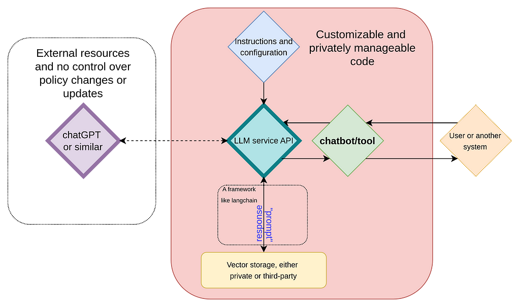
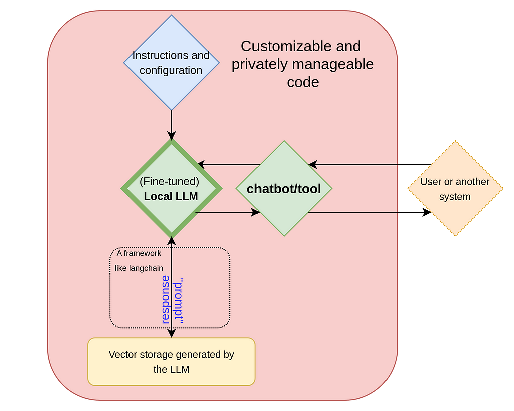
In one of our previous entries we explored the key concepts behind LLMs and how they can be used to create customized chatbots or tools with frameworks such as Langchain (see Fig. 1). In such schemes, while data can be protected by using synthetic data or obfuscation, we still must send data externally a third party and have no control over any changes in the model, its policies, or even its availability. A solution is simply to run an LLM on a private server (see Fig. 2). This approach ensures full privacy and mitigates the dependency on external service providers.
Concerns about implementing LLMs privately include costs, power consumption, and speed. In this exercise, we get LLama 3.1 running while varying the 1. framework (tools) and 2. degrees of quantization and compare the ease of use of the frameworks, the resultant performance in terms of speed, and power consumption. Understanding these trade-offs is essential for anyone looking to harness the full potential of AI while retaining control over their data and resources.
Fig. 1 Diagram illustrating a typical backend setup for chatbots or tools, with ChatGPT (or similar models) functioning as the natural language processing engine. This setup relies on prompt engineering to customize responses.”
Fig. 2 Diagram of a fully private backend configuration where all components, including the large language model, are hosted on a secure server, ensuring complete control and privacy.
Quantization and GGUF Files
Before diving into our impressions of the tools we explored, let’s first discuss quantization and the GGUF format.
Quantization is a technique used to reduce the size of a model by converting weights and biases from high-precision floating-point values to lower-precision representations. LLMs benefit greatly from this approach, given their vast number of parameters. For example, the largest version of Llama 3.1 contains a staggering 405 billion parameters. Quantization can significantly reduce both memory usage and execution time, making these models more efficient to run across a variety of devices. For an in-depth explanation and nomenclature of quantization types, check out this great introduction. A conceptual overview can also be found here.
The GGUF format is used to store LLM models and has recently gained popularity for distributing and running quantized models. It is optimized for fast loading, reading, and saving. Unlike tensor-only formats, GGUF also stores model metadata in a standardized manner, making it easier for frameworks to support this format or even adopt it as the norm.
Tools and Models Analyzed
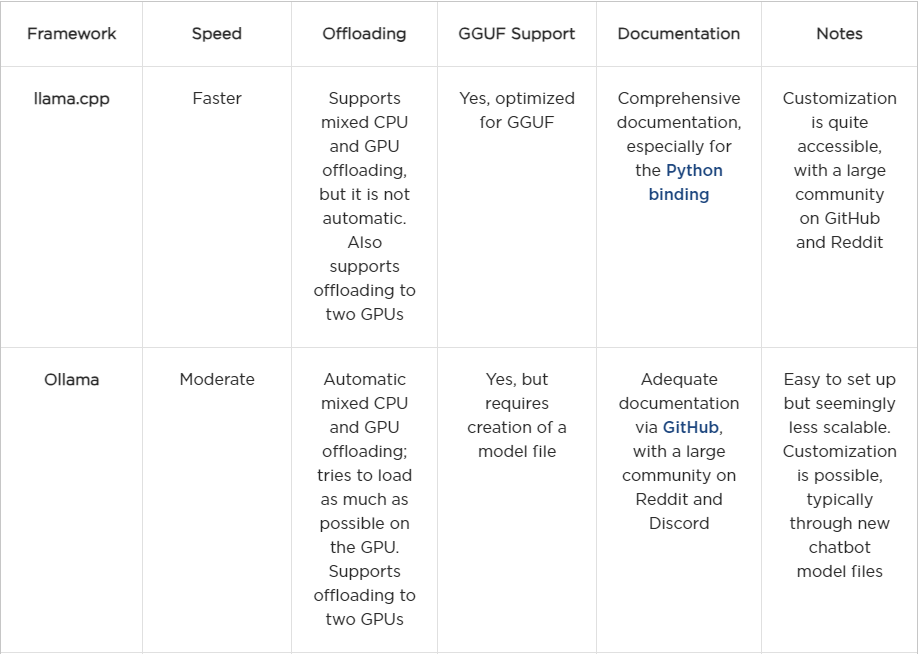
We explored four tools to run Llama models locally:
Our primary focus was on llama.cpp and Ollama, as these tools allowed us to deploy models quickly and efficiently right out of the box. Specifically, we explored their speed, energy cost, and overall performance. For the models, we primarily analyzed the quantized 8B and 70B Llama 3.1 versions, as they ran within a reasonable time frame.
First Impressions and Installation
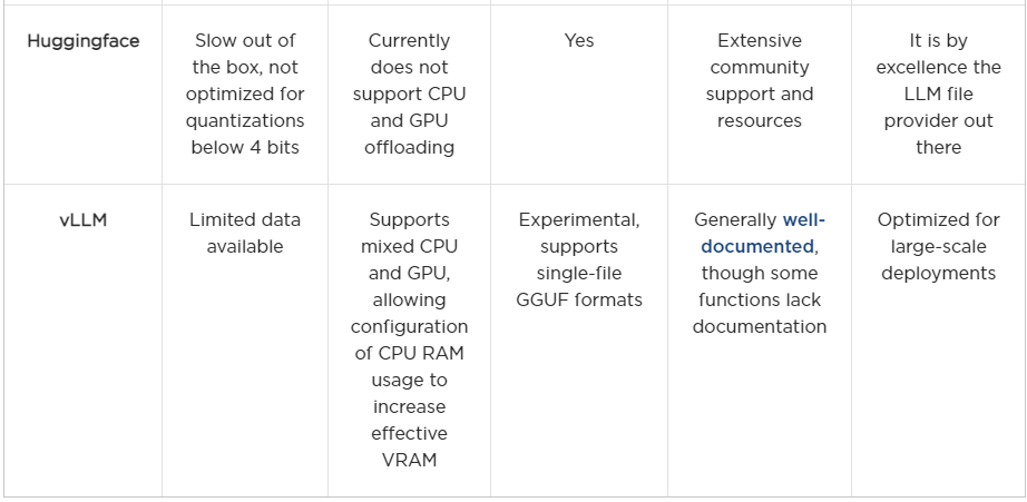
HuggingFace
HuggingFace’s transformers library and Hub are well-known and widely used in the community. They offer a wide range of models and tools, making them a popular choice for many developers. Its installation generally does not cause major problems once a proper environment is set up with Python. At the end of the day, the biggest benefit of Huggingface was its online hub, which allows for easy access to quantized models from many different providers. On the other hand, using the transformers library directly to load models, especially quantized ones, was rather tricky. Out of the box, the library seemingly directly dequantizes models, taking a great amount of ram and making it unfeasible to run in a local server.
Although Hugging Face supports 4- and 8-bit quantization and dequantization with bitsandbytes, our initial impression is that further optimization is needed. Efficient inference may simply not be its primary focus. Nonetheless, Hugging Face offers excellent documentation, a large community, and a robust framework for model training.
vLLM
Similar to Hugging Face, vLLM is easy to install with a properly configured Python environment. However, support for GGUF files is still highly experimental. While we were able to quickly set it up to run 8B models, scaling beyond that proved challenging, despite the excellent documentation.
Overall, we believe vLLM has great potential. However, we ultimately opted for the llama.cpp and Ollama frameworks for their more immediate compatibility and efficiency. To be fair, a more thorough investigation could have been conducted here, but given the immediate success we found with other libraries, we chose to focus on those.
Ollama
We found Ollama to be fantastic. Our initial impression is that it is a user-ready tool for inferring Llama models locally, with an ease-of-use that works right out of the box. Installing it for Mac and Linux users is straightforward, and a Windows version is currently in preview. Ollama automatically detects your hardware and manages model offloading between CPU and GPU seamlessly. It features its own model library, automatically downloading models and supporting GGUF files. Although its speed is slightly slower than llama.cpp, it performs well even on CPU-only setups and laptops.
For a quick start, once installed, running ollama run llama3.1:latest will load the latest 8B model in conversation mode directly from the command line.
One downside is that customizing models can be somewhat impractical, especially for advanced development. For instance, even adjusting the temperature requires creating a new chatbot instance, which in turn loads an installed model. While this is a minor inconvenience, it does facilitate the setup of customized chatbots — including other parameters and roles — within a single file. Overall, we believe Ollama serves as an effective local tool that mimics some of the key features of cloud services.
It is worth noting that Ollama runs as a service, at least on Linux machines, and offers handy, simple commands for monitoring which models are running and where they’re offloaded, with the ability to stop them instantly if needed. One challenge the community has faced is configuring certain aspects, such as where models are stored, which requires technical knowledge of Linux systems. While this may not pose a problem for end-users, it perhaps slightly hurts the tool’s practicality for advanced development purposes.
llama.cpp
llama.cpp emerged as our favorite tool during this analysis. As stated in its repository, it is designed for running inference on large language models with minimal setup and cutting-edge performance. Like Ollama, it supports offloading models between CPU and GPU, though this is not available straight out of the box. To enable GPU support, you must compile the tool with the appropriate flags — specifically, GGML_CUDA=on. We recommend using the latest version of the CUDA toolkit, as older versions may not be compatible.
The tool can be installed as a standalone by pulling from the repository and compiling, which provides a convenient command-line client for running models. For instance, you can execute llama-cli -p ‘you are a useful assistant’ -m Meta-Llama-3-8B-Instruct.Q8_0.gguf -cnv. Here, the final flag enables conversation mode directly from the command line. llama-cli offers various customization options, such as adjusting the context size, repetition penalty, and temperature, and it also supports GPU offloading options.
Similar to Ollama, llama.cpp has a Python binding which can be installed via pip install llama-cpp-python. This Python library allows for significant customization, making it easy for developers to tailor models to specific client needs. However, just as with the standalone version, the Python binding requires compilation with the appropriate flags to enable GPU support.
One minor downside is that the tool doesn’t yet support automatic CPU-GPU offloading. Instead, users need to manually specify how many layers to offload onto the GPU, with the remainder going to the CPU. While this requires some fine-tuning, it is a straightforward, manageable step.
For environments with multiple GPUs, like ours, llama.cpp provides two split modes: row mode and layer mode. In row mode, one GPU handles small tensors and intermediate results, while in layer mode, layers are divided across GPUs. In our tests, both modes delivered comparable performance (see analysis below).
Our Analysis
► From now on, results concern only llama.cpp and Ollama.
We conducted an analysis of the speed and power consumption of the 70B and 8B Llama 3.1 models using Ollama and llama.cpp. Specifically, we examined the speed and power consumption per token for each model across various quantizations available in Quant Factory.
To carry out this analysis, we developed a small application to evaluate the models once the tool was selected. During inference, we recorded metrics such as speed (tokens per second), total tokens generated, temperature, number of layers loaded on GPUs, and the quality rating of the response. Additionally, we measured the power consumption of the GPU during model execution. A script was used to monitor GPU power usage (via nvidia-smi) immediately after each token was generated. Once inference concluded, we computed the average power consumption based on these readings. Since we focused on models that could fully fit into GPU memory, we only measured GPU power consumption.
Additionally, the experiments were conducted with a variety of prompts to ensure different output sizes, thus, the data encompass a wide range of scenarios.
Hardware and Software Setup
We used a pretty decent server with the following features:
CPU: AMD Ryzen Threadripper PRO 7965WX 24-Cores @ 48x 5.362GHz.
GPU: 2x NVIDIA GeForce RTX 4090.
RAM: 515276MiB-
OS: Pop 22.04 jammy.
Kernel: x86_64 Linux 6.9.3–76060903-generic.
The retail cost of this setup was somewhere around $15,000 USD. We chose such a setup because it is a decent server that, while nowhere near as powerful as dedicated, high-end AI servers with 8 or more GPUs, is still quite functional and representative of what many of our clients might choose. We have found many clients hesitant to invest in high-end servers out of the gate, and this setup is a good compromise between cost and performance.
Speed
Let us first focus on speed. Below, we present several box-whisker plots depicting speed data for several quantizations. The name of each model starts with its quantization level; so for example “Q4” means a 4-bit quantization. Again, a LOWER quantization level rounds more, reducing size and quality but increasing speed.
► Technical Issue 1 (A Reminder of Box-Whisker Plots): Box-whisker plots display the median, the first and third quartiles, as well as the minimum and maximum data points. The whiskers extend to the most extreme points not classified as outliers, while outliers are plotted individually. Outliers are defined as data points that fall outside the range of Q1 − 1.5 × IQR and Q3 + 1.5 × IQR, where Q1 and Q3 represent the first and third quartiles, respectively. The interquartile range (IQR) is calculated as IQR = Q3 − Q1.
llama.cpp
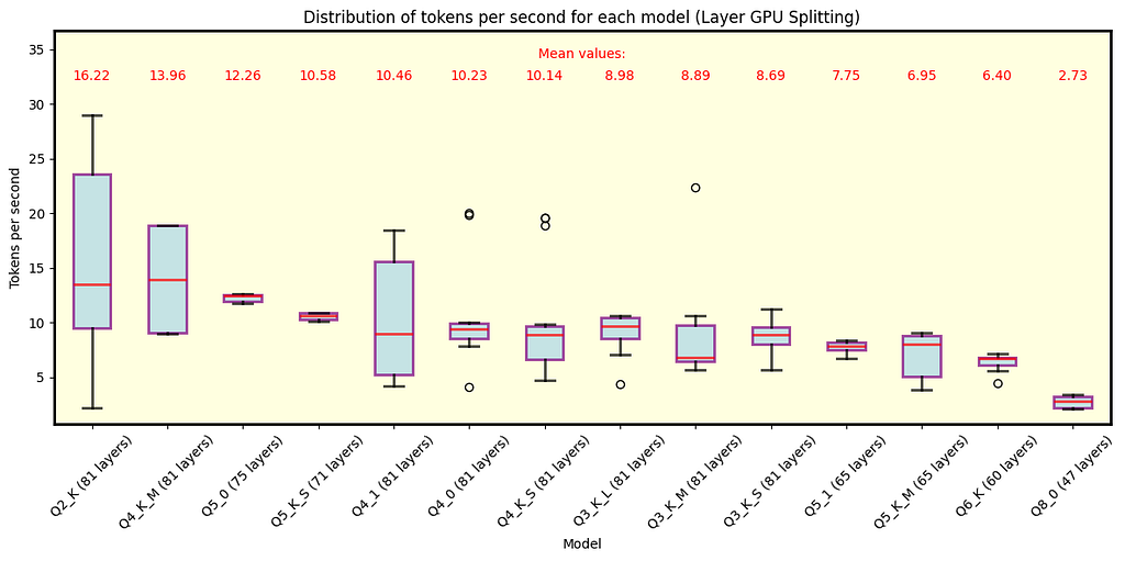
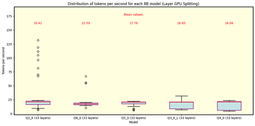
Below are the plots for llama.cpp. Fig. 3 shows the results for all Llama 3.1 models with 70B parameters available in QuantFactory, while Fig. 4 depicts some of the models with 8B parameters available here. 70B models can offload up to 81 layers onto the GPU while 8B models up to 33. For 70B, offloading all layers is not feasible for Q5 quantization and finer. Each quantization type includes the number of layers offloaded onto the GPU in parentheses. As expected, coarser quantization yields the best speed performance. Since row split mode performs similarly, we focus on layer split mode here.
Fig. 3 Llama 3.1 models with 70B parameters running under llama.cpp with split mode layer. As expected, coarser quantization provides the best speed. The number of layers offloaded onto the GPU is shown in parentheses next to each quantization type. Models with Q5 and finer quantizations do not fully fit into VRAM.
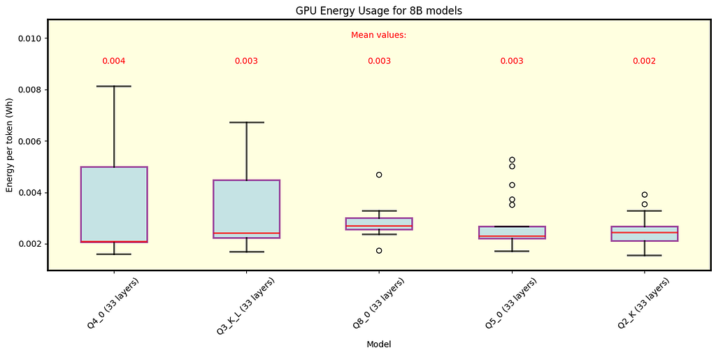
Fig. 4 Llama 3.1 models with 8B parameters running under llama.cpp using split mode layer. In this case, the model fits within the GPU memory for all quantization types, with coarser quantization resulting in the fastest speeds. Note that high speeds are outliers, while the overall trend hovers around 20 tokens per second for Q2_K.
Key Observations
During inference we observed some high speed events (especially in 8B Q2_K), this is where gathering data and understanding its distribution is crucial, as it turns out that those events are quite rare.
As expected, coarser quantization types yield the best speed performance. This is because the model size is reduced, allowing for faster execution.
The results concerning 70B models that do not fully fit into VRAM must be taken with caution, as using the CPU too could cause a bottleneck. Thus, the reported speed may not be the best representation of the model’s performance in those cases.
Ollama
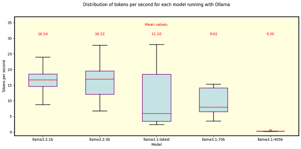
We executed the same analysis for Ollama. Fig. 5 shows the results for the default Llama 3.1 and 3.2 models that Ollama automatically downloads. All of them fit in the GPU memory except for the 405B model.
Fig. 5 Llama 3.1 and 3.2 models running under Ollama. These are the default models when using Ollama. All 3.1 models — specifically 405B, 70B, and 8B (labeled as “latest”) — use Q4_0 quantization, while the 3.2 models use Q8_0 (1B) and Q4_K_M (3B).
Key Observations
We can compare the 70B Q4_0 model across Ollama and llama.cpp, with Ollama exhibiting a slightly slower speed.
Similarly, the 8B Q4_0 model is slower under Ollama compared to its llama.cpp counterpart, with a more pronounced difference — llama.cpp processes about five more tokens per second on average.
Summary of Analyzed Frameworks
► Before discussing power consumption and rentability, let’s summarize the frameworks we analyzed up to this point.
Power Consumption and Rentability
This analysis is particularly relevant to models that fit all layers into GPU memory, as we only measured the power consumption of two RTX 4090 cards. Nonetheless, it is worth noting that the CPU used in these tests has a TDP of 350 W, which provides an estimate of its power draw at maximum load. If the entire model is loaded onto the GPU, the CPU likely maintains a power consumption close to idle levels.
To estimate energy consumption per token, we use the following parameters: tokens per second (NT) and power drawn by both GPUs (P) measured in watts. By calculating P/NT, we obtain the energy consumption per token in watt-seconds. Dividing this by 3600 gives the energy usage per token in Wh, which is more commonly referenced.
llama.cpp
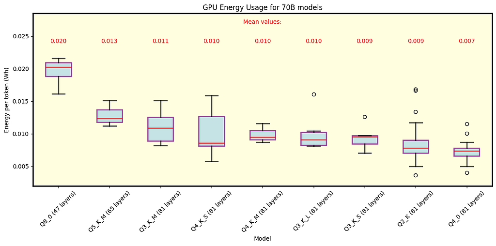
Below are the results for llama.cpp. Fig. 6 illustrates the energy consumption for 70B models, while Fig. 7 focuses on 8B models. These figures present energy consumption data for each quantization type, with average values shown in the legend.
Fig. 6 Energy per token for various quantizations of Llama 3.1 models with 70B parameters under llama.cpp. Both row and layer split modes are shown. Results are relevant only for models that fit all 81 layers in GPU memory.
Fig. 7 Energy per token for various quantizations of Llama 3.1 models with 8B parameters under llama.cpp. Both row and layer split modes are shown. All models exhibit similar average consumption.
Ollama
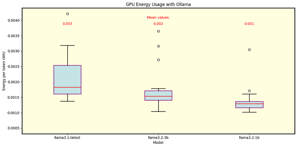
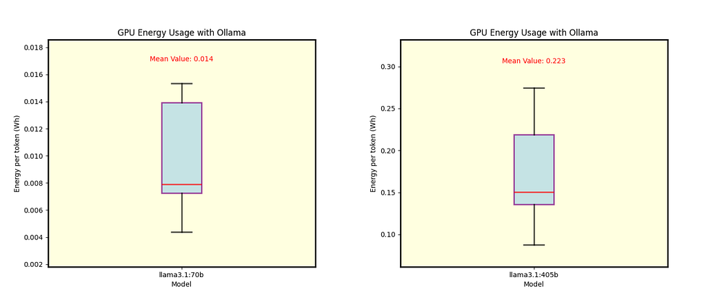
We also analyzed the energy consumption for Ollama. Fig. 8 displays results for Llama 3.1 8B (Q4_0 quantization) and Llama 3.2 1B and 3B (Q8_0 and Q4_K_M quantizations, respectively). Fig. 9 shows separate energy consumption for the 70B and 405B models, both with Q4_0 quantization.
Fig. 8 Energy per token for Llama 3.1 8B (Q4_0 quantization) and Llama 3.2 1B and 3B models (Q8_0 and Q4_K_M quantizations, respectively) under Ollama.
Fig. 9 Energy per token for Llama 3.1 70B (left) and Llama 3.1 405B (right), both using Q4_0 quantization under Ollama.
Summary of Costs
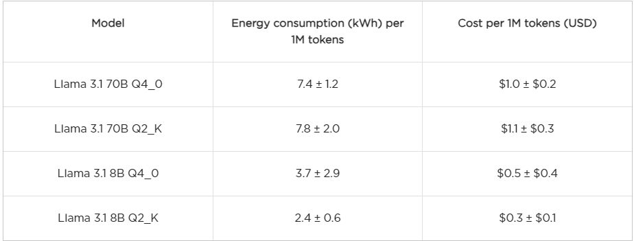
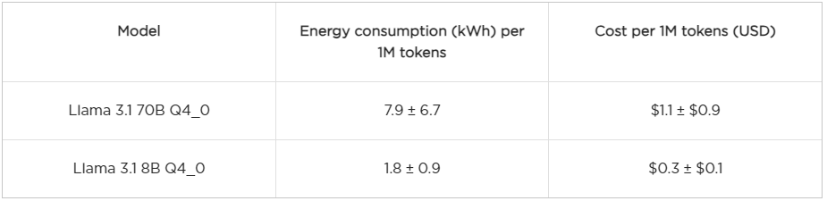
Instead of discussing each model individually, we will focus on those models that are comparable across llama.cpp and Ollama, as well of models with Q2_K quantization under llama.cpp, since it is the coarsest quantization explored here. To give a good idea of the costs, we show in the table below estimations of the energy consumption per one million generated tokens (1M) and the cost in USD. The cost is calculated based on the average electricity price in Texas, which is $0.14 per kWh according to this source. For a reference, the current pricing of GPT-4o is at least of $5 USD per 1M tokens and $0.3 USD per 1M tokens for GPT-o mini.
llama.cpp
Ollama
Key Observations
Using Llama 3.1 70B models with Q4_0, there is not much difference in the energy consumption between llama.cpp and Ollama.
For the 8B model llama.cpp spends more energy than Ollama.
Consider that the costs depicted here could be seen as a lower bound of the “bare costs” of running the models. Other costs, such as operation, maintenance, equipment costs and profit, are not included in this analysis.
The estimations suggest that operating LLMs on private servers can be cost-effective compared to cloud services. In particular, comparing Llama 8B with GPT-45o mini and Llama 70B with GPT-4o models seem to be a potential good deal under the right circumstances.
► Technical Issue 2 (Cost Estimation): For most models, the estimation of energy consumption per 1M tokens (and its variability) is given by the “median ± IQR” prescription, where IQR stands for interquartile range. Only for the Llama 3.1 8B Q4_0 model do we use the “mean ± STD” approach, with STD representing standard deviation. These choices are not arbitrary; all models except for Llama 3.1 8B Q4_0 exhibit outliers, making the median and IQR more robust estimators in those cases. Additionally, these choices help prevent negative values for costs. In most instances, when both approaches yield the same central tendency, they provide very similar results.
Final Word
Image by Meta AI
The analysis of speed and power consumption across different models and tools is only part of the broader picture. We observed that lightweight or heavily quantized models often struggled with reliability; hallucinations became more frequent as chat histories grew or tasks turned repetitive. This isn’t unexpected — smaller models don’t capture the extensive complexity of larger models. To counter these limitations, settings like repetition penalties and temperature adjustments can improve outputs. On the other hand, larger models like the 70B consistently showed strong performance with minimal hallucinations. However, since even the biggest models aren’t entirely free from inaccuracies, responsible and trustworthy use often involves integrating these models with additional tools, such as LangChain and vector databases. Although we didn’t explore specific task performance here, these integrations are key for minimizing hallucinations and enhancing model reliability.
In conclusion, running LLMs on private servers can provide a competitive alternative to LLMs as a service, with cost advantages and opportunities for customization. Both private and service-based options have their merits, and at Austin Ai, we specialize in implementing solutions that suit your needs, whether that means leveraging private servers, cloud services, or a hybrid approach.
Amazon Bedrock has launched a capability that organizations can use to tag on-demand models and monitor associated costs. Organizations can now label all Amazon Bedrock models with AWS cost allocation tags, aligning usage to specific organizational taxonomies such as cost centers, business units, and applications.
In this post, we discuss how to use AWS to support a decentralized clinical trial across the four main pillars of a decentralized clinical trial (virtual trials, personalized patient engagement, patient-centric trial design, and centralized data management). By exploring these AWS powered alternatives, we aim to demonstrate how organizations can drive progress towards more environmentally friendly clinical research practices.
Lessons Learned from the Worst Tech Job Market in 20 Years
Long Story Short. . .
. . . this job market is tough. Like, really tough. We all know what a roller coaster the past few years have been, particularly for those working in tech. We went from record-breaking salaries to hiring freezes and layoffs, all within a matter of months. 2023 saw the second-highest number of tech layoffs on record, surpassed only by the dot-com crash in 2001. While hiring in other sectors has remained resilient, the current tech job market is considered by many to be the worst since the turn of the century.
The impact of multiple rounds of layoffs has led to an influx of tech workers applying for a smaller number of open roles. Couple this with the immensely unpopular return-to-office mandates imposed by many large employers, and just about everyone is looking for a new job. This has led to increased competition for fewer roles, with salaries and perks that appear to be on the decline. Employers can afford to be pickier, and the interview process has become longer and more complex.
Applicant tracking systems and AI resume screeners have become the norm, creating a loop where it’s easy to apply to hundreds of jobs, but almost impossible to get your resume seen by a real person. Many of these vacancies may not even be ‘real’ jobs, with some companies posting positions that will never be filled.
In short, this job market has been a nightmare for tech workers. I tracked my experience looking for a new job for three months, aiming to take a more data-driven approach to the process. I applied to 443 positions, received 17 follow-up requests, interviewed with 13 companies, and ultimately landed one job offer. The insights from the analysis of this job search data can be used to more efficiently focus time and energy while navigating this completely bonkers job market.
Job Boards Matter
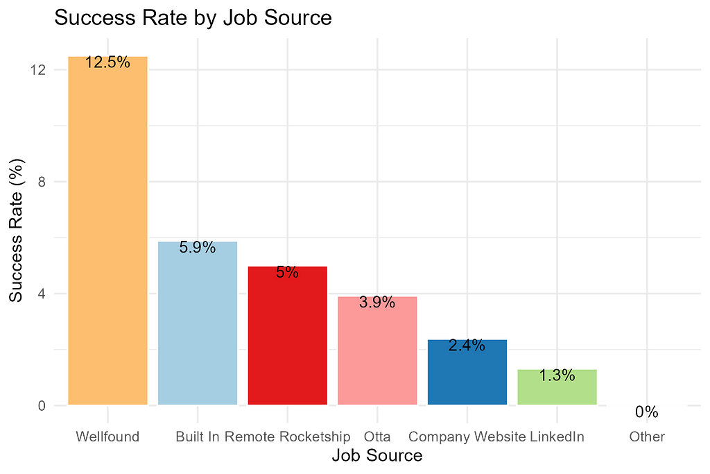
LinkedIn is, by far, the easiest and most popular way to find and apply for positions. But here is my hot take: Don’t use LinkedIn to apply for jobs. Over 1/3 of my applications were sent through LinkedIn, but only two of my interview invitations came from those applications — that’s a 1.3% success rate.
It’s easy to find and apply to jobs on LinkedIn, but quantity is no substitute for quality.
If you don’t already know, for jobs that you apply to through the ‘Easy Apply’ feature, you can check to see if your application has been viewed. Each application will have a status indicator next to it, which can include: ‘Applied’ (your initial submission) and ‘Viewed’ (the employer has seen your application).
When I discovered this feature, I didn’t believe it at first, because I had to scroll pretty far through my history to find an application that had actually been viewed. On average, I applied to jobs within 1.4 days of their initial posting. Despite this, hardly any of my LinkedIn applications were ever even viewed by a real person. Out of 152 applications I sent through LinkedIn, I only received 2 interview invitations in response.
The smaller job sites proved to be better resources for finding quality jobs with companies more likely to respond.
Of all the job boards I used, I found that applications submitted to jobs posted on Wellfound, Built In, and Remote Rocketship had the highest success rates.
Customized Resumes Don’t Help
The prevailing advice is to customize your resume for each position you apply to. With this in mind, I set a goal of a 30% customization rate. I tried a few paid AI services but found them laughably ineffective, and they didn’t really save any time. I ended up using Overleaf’s LaTeX editor and manually updating my skills and job responsibilities based on each job description.
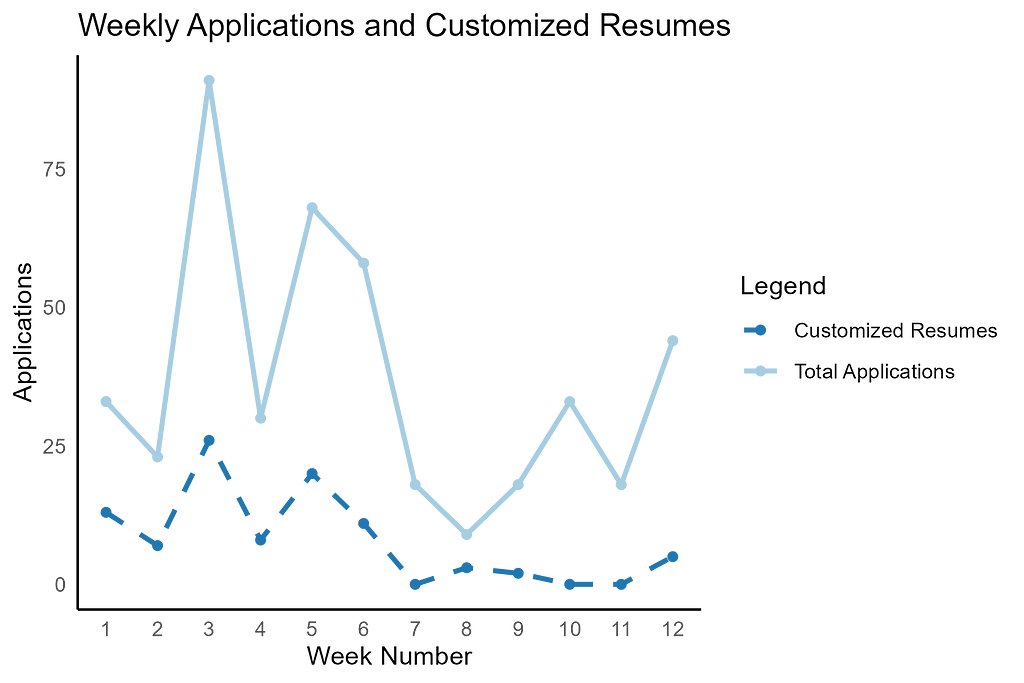
I submitted an average of 37 applications a week, of which 20%–30% were customized for the specific job.
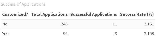
I maintained a customization rate of over 30% for the first month and a half, but it was extremely time consuming, and I got burnt out on the extra effort. Eventually, I went back to using a handful of generalized resumes that included the most commonly used tools and responsibilities and hoped that was good enough. When I compared the results of using the customized resumes versus the ‘good enough’ versions, surprisingly there was no real difference in rate of interview requests.
Customized resumes didn’t have a better outcome in regards to getting an interview.
I was shocked that putting in all the extra effort to customize my resume didn’t appear to make a difference in whether I received an interview invite. I even did a statistical analysis, which confirmed that fully customized resumes did not perform any better than generic versions. This finding could easily have saved me ten hours a week.
Job Titles and Self Confidence
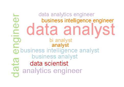
I have about four years of experience in analytics and engineering and applied to a wide range of job titles that fall under the data science umbrella.
These are the ten most common job titles I applied to during my search.
In my experience, jobs that include the word “analyst” are usually less technical and don’t pay quite as much as those ending in “scientist” or “engineer.” My academic background positions me well for one of those science or engineering jobs, but my work experience has been more towards the analyst level and scope. Because of this, I felt comfortably qualified for junior to mid-level analytics engineer and data analyst roles, while pure data science and data engineering opportunities felt like more of a stretch. Business analyst opportunities tend to be even less technical. The types of positions I applied for reflected my assumptions about my strength as a candidate and the competitiveness of the job market.
Most of my job applications were for entry to mid level data analyst positions.
If you had asked me what my career goals were, I would have told you landing a data science or engineering position was my dream. But I considered myself more qualified for data analyst roles, and so I spent the most time searching and applying for those opportunities.
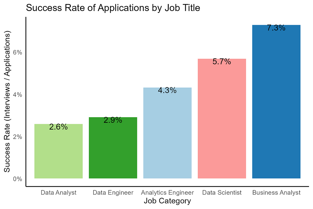
It turns out I was completely wrong. The success rate of my applications did not mirror my self-assessment. I was actually offered interviews for data science and data engineer positions at a higher rate than for data analyst roles. I had a 219% greater chance of landing an interview for a data science position than a data analyst role, but I applied to them 82% less often because I assumedI wouldn’t be successful.
I got a better response to positions that I applied to less often.
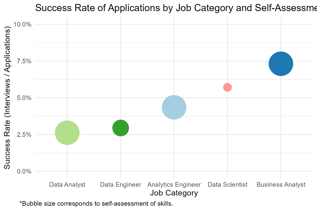
There seems to be no correlation between how I rated my qualifications for a job title and how often I got an interview relative to how many applications I submitted. I may have been sabotaging my own efforts by applying to fewer data science and engineering jobs because I lacked confidence in my skills.
How I rated my own qualifications did not reflect how successful I was at getting an interview.
Ghosting is Real
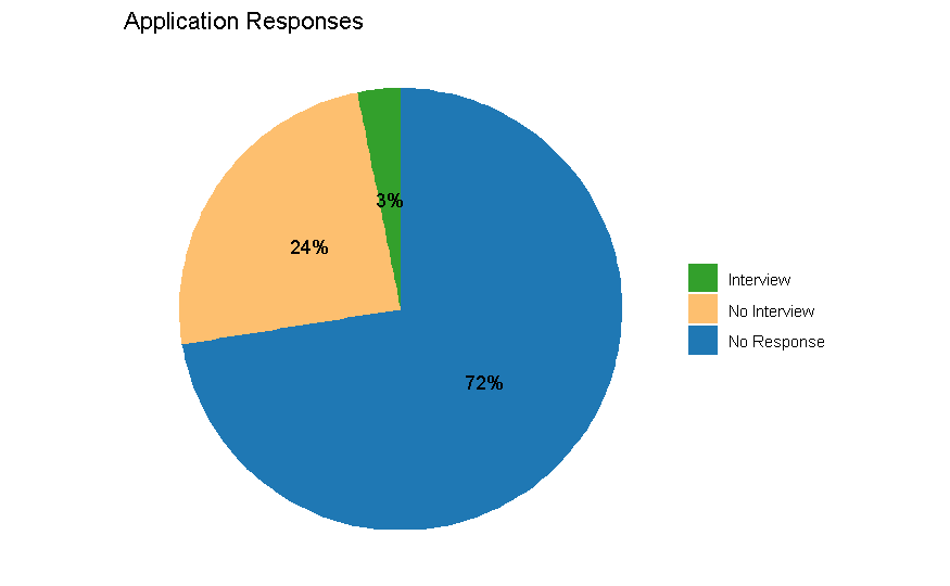
Out of all 443 job applications I submitted, I received just over 100 responses where the company declined to move forward with my candidacy. Eight of these were because the positions were canceled or put on hold. If you do the math, that means 72% of companies that I applied to never responded to my application at all. Job applications take a considerable amount of time, and it’s surprising how many companies don’t follow-up with candidates.
Most positions I applied to, I never heard back from. Only 3% of all applications resulted in an interview.
On average, companies responded 5 days faster when extending an interview invitation as opposed to a rejection. I observed an average 12.6 day response time for successful applications, compared to 17.9 days for declines. In most cases if it’s been more than two weeks since applying and you haven’t heard anything, that’s a good sign to move on and keep looking.
What I Learned
I did receive an offer in the third month of my search for a Business Intelligence Analyst position at a small company. I ended up declining the offer for reasons that I might just have to write a whole other blog about to explain. But in short, it wasn’t the right opportunity, and I chose to keep looking.
In a strange twist of fate, there was actually a second offer I received from an application I submitted a month before I started tracking this data. I applied for a data science position with the federal government in May, was called for an interview 4.5 months later in September, and after one 30-minute call with the hiring manager (which I thought I bombed), I got a job offer the next business day.
The experience of interviewing is invaluable, but even after all this practice, I still struggle with confidence and have trouble articulating my skills and abilities. Exploring this data analysis has helped me realize that even though I ultimately found a great job, I should continue to work on recognizing my strengths and accomplishments. Furthermore, almost all of my initial assumptions about where to find jobs, how to apply, or what roles to target turned out to be wrong. While my journey on this path is finally coming to an end, I hope the insights from my experience can also help others make more informed decisions on how to best use their time and energy.
Let this be the final lesson: You never know when doors will open for you. Keep your head up, keep trying, and stay positive. It’s a tough job market, but it won’t be like this forever. And if you are fortunate enough to have the resources to continue searching, never take a questionable offer. If you see red flags, don’t ignore them. Companies may have the upper hand right now, but that doesn’t mean you should compromise on what’s important to you. If it’s a bad fit, keep looking — other opportunities will come along. Never be afraid to put yourself out there, and always remind yourself of your worth. And for the final hot takeaway, stay off LinkedIn, apply for jobs even if you think they are a stretch, and don’t waste too much time customizing your resume!
All data visuals were created by the author using R. The full analysis and sample data set is available on GitHub.
Cruel Summer was originally published in Towards Data Science on Medium, where people are continuing the conversation by highlighting and responding to this story.
This post covers the steps to configure the Amazon Q Business Google Drive connector, including authentication setup and verifying the secure indexing of your Google Drive content.
Druva enables cyber, data, and operational resilience for thousands of enterprises, and is trusted by 60 of the Fortune 500. In this post, we show how Druva approached natural language querying (NLQ)—asking questions in English and getting tabular data as answers—using Amazon Bedrock, the challenges they faced, sample prompts, and key learnings.
I’ve been having a lot of fun in my daily work recently experimenting with models from the Hugging Face catalog, and I thought this might be a good time to share what I’ve learned and give readers some tips for how to apply these models with a minimum of stress.
My specific task recently has involved looking at blobs of unstructured text data (think memos, emails, free text comment fields, etc) and classifying them according to categories that are relevant to a business use case. There are a ton of ways you can do this, and I’ve been exploring as many as I can feasibly do, including simple stuff like pattern matching and lexicon search, but also expanding to using pre-built neural network models for a number of different functionalities, and I’ve been moderately pleased with the results.
I think the best strategy is to incorporate multiple techniques, in some form of ensembling, to get the best of the options. I don’t trust these models necessarily to get things right often enough (and definitely not consistently enough) to use them solo, but when combined with more basic techniques they can add to the signal.
Choosing the use case
For me, as I’ve mentioned, the task is just to take blobs of text, usually written by a human, with no consistent format or schema, and try to figure out what categories apply to that text. I’ve taken a few different approaches, outside of the analysis methods mentioned earlier, to do that, and these range from very low effort to somewhat more work on my part. These are three of the strategies that I’ve tested so far.
Ask the model to choose the category (zero-shot classification — I’ll use this as an example later on in this article)
Use a named entity recognition model to find key objects referenced in the text, and make classification based on that
Ask the model to summarize the text, then apply other techniques to make classification based on the summary
Finding the models
This is some of the most fun — looking through the Hugging Face catalog for models! At https://huggingface.co/models you can see a gigantic assortment of the models available, which have been added to the catalog by users. I have a few tips and pieces of advice for how to select wisely.
Look at the download and like numbers, and don’t choose something that has not been tried and tested by a decent number of other users. You can also check the Community tab on each model page to see if users are discussing challenges or reporting bugs.
Investigate who uploaded the model, if possible, and determine if you find them trustworthy. This person who trained or tuned the model may or may not know what they’re doing, and the quality of your results will depend on them!
Read the documentation closely, and skip models with little or no documentation. You’ll struggle to use them effectively anyway.
Use the filters on the side of the page to narrow down to models suited to your task. The volume of choices can be overwhelming, but they are well categorized to help you find what you need.
Most model cards offer a quick test you can run to see the model’s behavior, but keep in mind that this is just one example and it’s probably one that was chosen because the model’s good at that and finds this case pretty easy.
Incorporating into your code
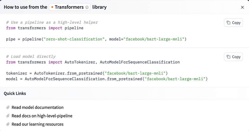
Once you’ve found a model you’d like to try, it’s easy to get going- click the “Use this Model” button on the top right of the Model Card page, and you’ll see the choices for how to implement. If you choose the Transformers option, you’ll get some instructions that look like this.
Screenshot taken by author
If a model you’ve selected is not supported by the Transformers library, there may be other techniques listed, like TF-Keras, scikit-learn, or more, but all should show instructions and sample code for easy use when you click that button.
In my experiments, all the models were supported by Transformers, so I had a mostly easy time getting them running, just by following these steps. If you find that you have questions, you can also look at the deeper documentation and see full API details for the Transformers library and the different classes it offers. I’ve definitely spent some time looking at these docs for specific classes when optimizing, but to get the basics up and running you shouldn’t really need to.
Preparing inference data
Ok, so you’ve picked out a model that you want to try. Do you already have data? If not, I have been using several publicly available datasets for this experimentation, mainly from Kaggle, and you can find lots of useful datasets there as well. In addition, Hugging Face also has a dataset catalog you can check out, but in my experience it’s not as easy to search or to understand the data contents over there (just not as much documentation).
Once you pick a dataset of unstructured text data, loading it to use in these models isn’t that difficult. Load your model and your tokenizer (from the docs provided on Hugging Face as noted above) and pass all this to the pipeline function from the transformers library. You’ll loop over your blobs of text in a list or pandas Series and pass them to the model function. This is essentially the same for whatever kind of task you’re doing, although for zero-shot classification you also need to provide a candidate label or list of labels, as I’ll show below.
Code Example
So, let’s take a closer look at zero-shot classification. As I’ve noted above, this involves using a pretrained model to classify a text according to categories that it hasn’t been specifically trained on, in the hopes that it can use its learned semantic embeddings to measure similarities between the text and the label terms.
from transformers import AutoModelForSequenceClassification from transformers import AutoTokenizer from transformers import pipeline
all_results = [] for text in list_of_texts: prob = self.classifier(text, label_list, multi_label=True, use_fast=True) results_dict = {x: y for x, y in zip(prob["labels"], prob["scores"])} all_results.append(results_dict)
This will return you a list of dicts, and each of those dicts will contain keys for the possible labels, and the values are the probability of each label. You don’t have to use the pipeline as I’ve done here, but it makes multi-label zero shot a lot easier than manually writing that code, and it returns results that are easy to interpret and work with.
If you prefer to not use the pipeline, you can do something like this instead, but you’ll have to run it once for each label. Notice how the processing of the logits resulting from the model run needs to be specified so that you get human-interpretable output. Also, you still need to load the tokenizer and the model as described above.
def run_zero_shot_classifier(text, label): hypothesis = f"This example is related to {label}."
x = tokenizer.encode( text, hypothesis, return_tensors="pt", truncation_strategy="only_first" )
label_list = ['News', 'Science', 'Art'] all_results = [] for text in list_of_texts: for label in label_list: result = run_zero_shot_classifier(text, label) all_results.append(result)
To tune, or not?
You probably have noticed that I haven’t talked about fine tuning the models myself for this project — that’s true. I may do this in future, but I’m limited by the fact that I have minimal labeled training data to work with at this time. I can use semisupervised techniques or bootstrap a labeled training set, but this whole experiment has been to see how far I can get with straight off-the-shelf models. I do have a few small labeled data samples, for use in testing the models’ performance, but that’s nowhere near the same volume of data I will need to tune the models.
Performance has been an interesting problem, as I’ve run all my experiments on my local laptop so far. Naturally, using these models from Hugging Face will be much more compute intensive and slower than the basic strategies like regex and lexicon search, but it provides signal that can’t really be achieved any other way, so finding ways to optimize can be worthwhile. All these models are GPU enabled, and it’s very easy to push them to be run on GPU. (If you want to try it on GPU quickly, review the code I’ve shown above, and where you see “cpu” substitute in “cuda” if you have a GPU available in your programming environment.) Keep in mind that using GPUs from cloud providers is not cheap, however, so prioritize accordingly and decide if more speed is worth the price.
Most of the time, using the GPU is much more important for training (keep it in mind if you choose to fine tune) but less vital for inference. I’m not digging in to more details about optimization here, but you’ll want to consider parallelism as well if this is important to you- both data parallelism and actual training/compute parallelism.
Testing and understanding output
We’ve run the model! Results are here. I have a few closing tips for how to review the output and actually apply it to business questions.
Don’t trust the model output blindly, but run rigorous tests and evaluate performance. Just because a transformer model does well on a certain text blob, or is able to correctly match text to a certain label regularly, doesn’t mean this is generalizable result. Use lots of different examples and different kinds of text to prove the performance is going to be sufficient.
If you feel confident in the model and want to use it in a production setting, track and log the model’s behavior. This is just good practice for any model in production, but you should keep the results it has produced alongside the inputs you gave it, so you can continually check up on it and make sure the performance doesn’t decline. This is more important for these kinds of deep learning models because we don’t have as much interpretability of why and how the model is coming up with its inferences. It’s dangerous to make too many assumptions about the inner workings of the model.
As I mentioned earlier, I like using these kinds of model output as part of a larger pool of techniques, combining them in ensemble strategies — that way I’m not only relying on one approach, but I do get the signal those inferences can provide.
I hope this overview is useful for those of you getting started with pre-trained models for text (or other mode) analysis — good luck!
We use cookies on our website to give you the most relevant experience by remembering your preferences and repeat visits. By clicking “Accept”, you consent to the use of ALL the cookies.
This website uses cookies to improve your experience while you navigate through the website. Out of these, the cookies that are categorized as necessary are stored on your browser as they are essential for the working of basic functionalities of the website. We also use third-party cookies that help us analyze and understand how you use this website. These cookies will be stored in your browser only with your consent. You also have the option to opt-out of these cookies. But opting out of some of these cookies may affect your browsing experience.
Necessary cookies are absolutely essential for the website to function properly. These cookies ensure basic functionalities and security features of the website, anonymously.
Cookie
Duration
Description
cookielawinfo-checkbox-analytics
11 months
This cookie is set by GDPR Cookie Consent plugin. The cookie is used to store the user consent for the cookies in the category "Analytics".
cookielawinfo-checkbox-functional
11 months
The cookie is set by GDPR cookie consent to record the user consent for the cookies in the category "Functional".
cookielawinfo-checkbox-necessary
11 months
This cookie is set by GDPR Cookie Consent plugin. The cookies is used to store the user consent for the cookies in the category "Necessary".
cookielawinfo-checkbox-others
11 months
This cookie is set by GDPR Cookie Consent plugin. The cookie is used to store the user consent for the cookies in the category "Other.
cookielawinfo-checkbox-performance
11 months
This cookie is set by GDPR Cookie Consent plugin. The cookie is used to store the user consent for the cookies in the category "Performance".
viewed_cookie_policy
11 months
The cookie is set by the GDPR Cookie Consent plugin and is used to store whether or not user has consented to the use of cookies. It does not store any personal data.
Functional cookies help to perform certain functionalities like sharing the content of the website on social media platforms, collect feedbacks, and other third-party features.
Performance cookies are used to understand and analyze the key performance indexes of the website which helps in delivering a better user experience for the visitors.
Analytical cookies are used to understand how visitors interact with the website. These cookies help provide information on metrics the number of visitors, bounce rate, traffic source, etc.
Advertisement cookies are used to provide visitors with relevant ads and marketing campaigns. These cookies track visitors across websites and collect information to provide customized ads.