
An article on the most common LLM development challenges I’ve encountered, effective mitigation strategies, and a career-defining…
Originally appeared here:
Overcoming LLM Challenges in Healthcare: Practical Strategies for Development in Production

An article on the most common LLM development challenges I’ve encountered, effective mitigation strategies, and a career-defining…
Originally appeared here:
Overcoming LLM Challenges in Healthcare: Practical Strategies for Development in Production


How to turn vector elevation lines into a grid — and build it from Lego
Originally appeared here:
Rasterizing Vector Data in Python
Go Here to Read this Fast! Rasterizing Vector Data in Python

Remember the days when classifying text meant embarking on a machine learning journey? If you’ve been in the ML space long enough, you’ve probably witnessed at least one team disappear down the rabbit hole of building the “perfect” text classification system. The story usually goes something like this:
For years, text classification has fallen into the realm of classic ML. Early in my career, I remember training a support vector machine (SVM) for email classification. Lots of preprocessing, iteration, data collection, and labeling.
But here’s the twist: it’s 2024, and generative AI models can “generally” classify text out of the box! You can build a robust ticket classification system without, collecting thousands of labeled training examples, managing ML training pipelines, or maintaining custom models.
In this post, we’ll go over how to setup a Jira ticket classification system using large language models on Amazon Bedrock and other AWS services.
DISCLAIMER: I am a GenAI Architect at AWS and my opinions are my own.
A common ask from companies is to understand how teams spend their time. Jira has tagging features, but it can sometimes fall short through human error or lack of granularity. By doing this exercise, organizations can get better insights into their team activities, enabling data-driven decisions about resource allocation, project investment, and deprecation.
Traditional ML models and smaller transformers like BERT need hundreds (or thousands) of labeled examples, while LLMs can classify text out of the box. In our Jira ticket classification tests, a prompt-engineering approach matched or beat traditional ML models, processing 10k+ annual tickets for ~$10/year using Claude Haiku (excluding other AWS Service costs). Also, prompts are easier to update than retraining models.
This github repo contains a sample application that connects to Jira Cloud, classifies tickets, and outputs them in a format that can be consumed by your favorite dashboarding tool (Tableu, Quicksight, or any other tool that supports CSVs).
Important Notice: This project deploys resources in your AWS environment using Terraform. You will incur costs for the AWS resources used. Please be aware of the pricing for services like Lambda, Bedrock, Glue, and S3 in your AWS region.
Pre Requisites
You’ll need to have terraform installed and the AWS CLI installed in the environment you want to deploy this code from
The architecture is pretty straight forward. You can find details below.
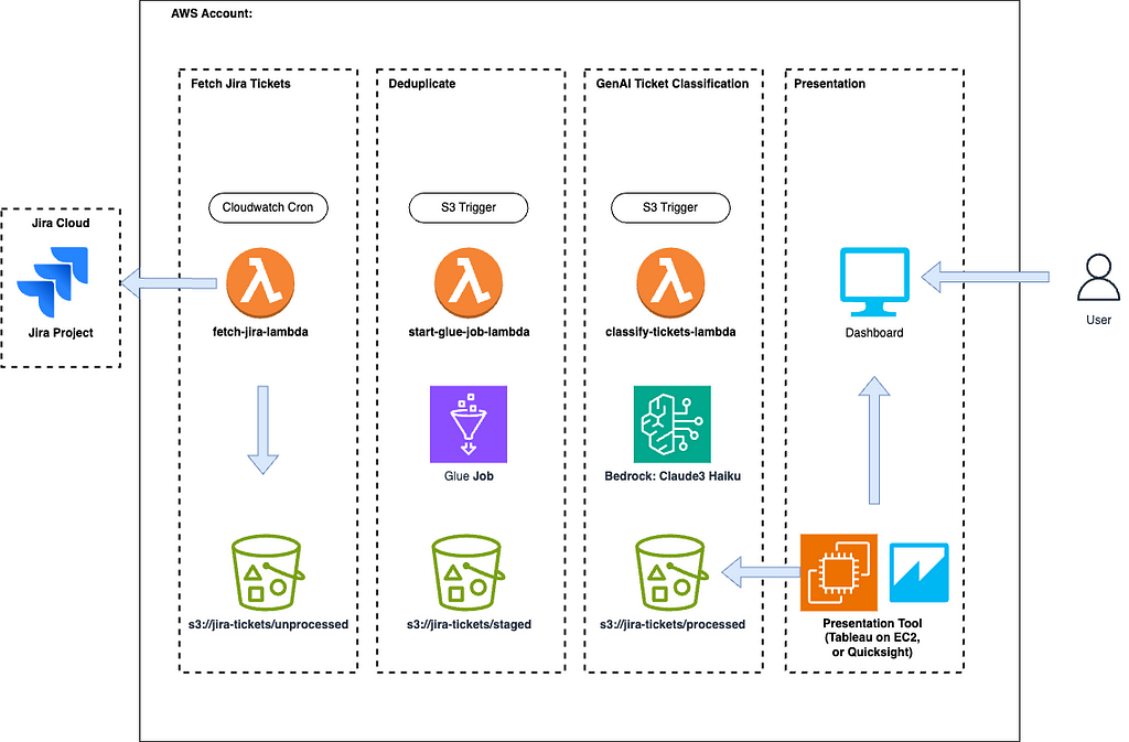
Step 1: An AWS Lambda function is triggered on a cron job to fetch jira tickets based on a time window. Those tickets are then formatted and pushed to an S3 bucket under the /unprocessed prefix.
Step 2: A Glue job is triggered off /unprocessed object puts. This runs a PySpark deduplication task to ensure no duplicate tickets make their way to the dashboard. The deduplicated tickets are then put to the /staged prefix. This is useful for cases where you manually upload tickets as well as rely on the automatic fetch. If you can ensure no duplicates, you can remove this step.
Step 3: A classification task is kicked off on the new tickets by calling Amazon Bedrock to classify the tickets based on a prompt to a large language model (LLM). After classification, the finished results are pushed to the /processed prefix. From here, you can pick up the processed CSV using any dashboarding tool you’d like that can consume a CSV.
To get started, clone the github repo above and move to the /terraform directory
$ git clone https://github.com/aws-samples/jira-ticket-classification.git

$ cd jira-ticket-classification/terraform
Run terraform init, plan, & apply. Make sure you have terraform installed on your computer and the AWS CLI configured.
$ terraform init

$ terraform plan

$ terraform apply
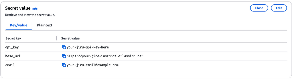
Once the infrastructure is deployed into your account, you can navigate to AWS Secrets Manager and update the secret with your Jira Cloud credentials. You’ll need an API key, base url, and email to enable the automatic pull
And that’s it!
You can (1) wait for the Cron to kick off an automatic fetch, (2) export the tickets to CSV and upload them to the /unprocessed S3 bucket prefix, or (3) manually trigger the Lambda function using a test.
Jira fetch uses a Lambda function with a Cloudwatch cron event to trigger it. The Lambda pulls in the AWS Secret and uses a get request in a while loop to retrieve paginated results until the JQL query completes:
def fetch_jira_issues(base_url, project_id, email, api_key):
    url = f"{base_url}/rest/api/3/search"

    # Calculate the date 8 days ago
    eight_days_ago = (datetime.now() - timedelta(days=8)).strftime("%Y-%m-%d")

    # Create JQL
    jql = f"project = {project_id} AND created >= '{eight_days_ago}' ORDER BY created DESC"

    # Pass into params of request.
    params = {
        "jql": jql,
        "startAt": 0
    }
    all_issues = []

    auth = HTTPBasicAuth(email, api_key)
    headers = {"Accept": "application/json"}

    while True:
        response = requests.get(url, headers=headers, params=params, auth=auth)
        if response.status_code != 200:
            raise Exception(f"Failed to fetch issues for project {project_id}: {response.text}")

        data = json.loads(response.text)
        issues = data['issues']
        all_issues.extend(issues)

        if len(all_issues) >= data['total']:
            break

        params['startAt'] = len(all_issues)

    return all_issues
It then creates a string representation of a CSV and uploads it into S3:
def upload_to_s3(csv_string, bucket, key):
    try:
        s3_client.put_object(
            Bucket=bucket,
            Key=key,
            Body=csv_string,
            ContentType='text/csv'
        )
    except Exception as e:
        raise Exception(f"Failed to upload CSV to S3: {str(e)}")
An S3 event on the /unprocessed prefix kicks off a second lambda that starts an AWS Glue job. This is useful when there’s multiple entry points that Jira tickets can enter the system through. For example, if you want to do a backfill.
import boto3

# Initialize Boto3 Glue client
glue_client = boto3.client('glue')

def handler(event, context):
    # Print event for debugging
    print(f"Received event: {json.dumps(event)}")

    # Get bucket name and object key (file name) from the S3 event
    try:
        s3_event = event['Records'][0]['s3']
        s3_bucket = s3_event['bucket']['name']
        s3_key = s3_event['object']['key']
    except KeyError as e:
        print(f"Error parsing S3 event: {str(e)}")
        raise

    response = glue_client.start_job_run(
        JobName=glue_job_name,
        Arguments={
            '--S3_BUCKET': s3_bucket,
            '--NEW_CSV_FILE': s3_key
        }
    )
The Glue job itself is written in PySpark and can be found in the code repo here. The important take away is that it does a leftanti join using the issue Ids on the items in the new CSV against all the Ids in the /staged CSVs.
The results are then pushed to the /staged prefix.
This is where it it gets interesting. As it turns out, using prompt engineering can perform on par, if not better, than a text classification model using a couple techniques.
Note: It’s important to validate your prompt using a human curated subset of classified / labelled tickets. You should run this prompt through the validation dataset to make sure it aligns with how you expect the tickets to be classified
SYSTEM_PROMPT = '''
You are a support ticket assistant. You are given fields of a Jira ticket and your task is to classify the ticket based on those fields

Below is the list of potential classifications along with descriptions of those classifications.
<classifications>
ACCESS_PERMISSIONS_REQUEST: Used when someone doesn't have the write permissions or can't log in to something or they can't get the correct IAM credentials to make a service work.
BUG_FIXING: Used when something is failing or a bug is found. Often times the descriptions include logs or technical information.
CREATING_UPDATING_OR_DEPRECATING_DOCUMENTATION: Used when documentation is out of date. Usually references documentation in the text.
MINOR_REQUEST: This is rarely used. Usually a bug fix but it's very minor. If it seems even remotely complicated use BUG_FIXING.
SUPPORT_TROUBLESHOOTING: Used when asking for support for some engineering event. Can also look like an automated ticket.
NEW_FEATURE_WORK: Usually describes a new feature ask or something that isn't operational.
</classifications>

The fields available and their descriptions are below.
<fields>
Summmary: This is a summary or title of the ticket
Description: The description of the issue in natural language. The majority of context needed to classify the text will come from this field
</fields>


<rules>
* It is possible that some fields may be empty in which case ignore them when classifying the ticket
* Think through your reasoning before making the classification and place your thought process in <thinking></thinking> tags. This is your space to think and reason about the ticket classificaiton.
* Once you have finished thinking, classify the ticket using ONLY the classifications listed above and place it in <answer></answer> tags.
</rules>'''

USER_PROMPT = '''
Using only the ticket fields below:

<summary_field>
{summary}
</summary_field>

<description_field>
{description}
</description_field>

Classify the ticket using ONLY 1 of the classifications listed in the system prompt. Remember to think step-by-step before classifying the ticket and place your thoughts in <thinking></thinking> tags.
When you are finished thinking, classify the ticket and place your answer in <answer></answer> tags. ONLY place the classifaction in the answer tags. Nothing else.
'''
We’ve added a helper class that threads the calls to Bedrock to speed things up:
import boto3
from concurrent.futures import ThreadPoolExecutor, as_completed
import re
from typing import List, Dict
from prompts import USER_PROMPT, SYSTEM_PROMPT

class TicketClassifier:
    SONNET_ID = "anthropic.claude-3-sonnet-20240229-v1:0"
    HAIKU_ID = "anthropic.claude-3-haiku-20240307-v1:0"
    HYPER_PARAMS = {"temperature": 0.35, "topP": .3}
    REASONING_PATTERN = r'<thinking>(.*?)</thinking>'
    CORRECTNESS_PATTERN = r'<answer>(.*?)</answer>'

    def __init__(self):
        self.bedrock = boto3.client('bedrock-runtime')

    def classify_tickets(self, tickets: List[Dict[str, str]]) -> List[Dict[str, str]]:
        prompts = [self._create_chat_payload(t) for t in tickets]
        responses = self._call_threaded(prompts, self._call_bedrock)
        formatted_responses = [self._format_results(r) for r in responses]
        return [{**d1, **d2} for d1, d2 in zip(tickets, formatted_responses)]

    def _call_bedrock(self, message_list: list[dict]) -> str:
        response = self.bedrock.converse(
            modelId=self.HAIKU_ID,
            messages=message_list,
            inferenceConfig=self.HYPER_PARAMS,
            system=[{"text": SYSTEM_PROMPT}]
        )
        return response['output']['message']['content'][0]['text']

    def _call_threaded(self, requests, function):
        future_to_position = {}
        with ThreadPoolExecutor(max_workers=5) as executor:
            for i, request in enumerate(requests):
                future = executor.submit(function, request)
                future_to_position[future] = i
            responses = [None] * len(requests)
            for future in as_completed(future_to_position):
                position = future_to_position[future]
                try:
                    response = future.result()
                    responses[position] = response
                except Exception as exc:
                    print(f"Request at position {position} generated an exception: {exc}")
                    responses[position] = None
        return responses

    def _create_chat_payload(self, ticket: dict) -> dict:
        user_prompt = USER_PROMPT.format(summary=ticket['Summary'], description=ticket['Description'])
        user_msg = {"role": "user", "content": [{"text": user_prompt}]}
        return [user_msg]

    def _format_results(self, model_response: str) -> dict:
        reasoning = self._extract_with_regex(model_response, self.REASONING_PATTERN)
        correctness = self._extract_with_regex(model_response, self.CORRECTNESS_PATTERN)
        return {'Model Answer': correctness, 'Reasoning': reasoning}

    @staticmethod
    def _extract_with_regex(response, regex):
        matches = re.search(regex, response, re.DOTALL)
        return matches.group(1).strip() if matches else None
Lastly, the classified tickets are converted to a CSV and uploaded to S3
import boto3
import io
import csv

s3 = boto3.client('s3')

def upload_csv(data: List[Dict[str, str]]) -> None:
      csv_buffer = io.StringIO()
      writer = csv.DictWriter(csv_buffer, fieldnames=data[0].keys())
      writer.writeheader()
      writer.writerows(data)

      current_time = datetime.now().strftime("%Y%m%d_%H%M%S")
      filename = f"processed/processed_{current_time}.csv"

      s3.put_object(
          Bucket=self.bucket_name,
          Key=filename,
          Body=csv_buffer.getvalue()
      )
The project is dashboard agnostic. Any popular tool/service will work as long as it can consume a CSV. Amazon Quicksight, Tableu or anything in between will do.
In this blog we discussed using Bedrock to automatically classify Jira tickets. These enriched tickets can then be used to create dashboards using various AWS Services or 3P tools. The takeaway, is that classifying text has become much simpler since the adoption of LLMs and what would have taken weeks can now be done in days.
If you enjoyed this article feel free to connect with me on LinkedIn
Classify Jira Tickets with GenAI On Amazon Bedrock was originally published in Towards Data Science on Medium, where people are continuing the conversation by highlighting and responding to this story.
Originally appeared here:
Classify Jira Tickets with GenAI On Amazon Bedrock
Go Here to Read this Fast! Classify Jira Tickets with GenAI On Amazon Bedrock

AI models, particularly Large Language Models (LLMs), need large amounts of GPU memory. For example, in the case of the LLaMA 3.1 model, released in July 2024, the memory requirements are:
In a full-sized machine learning model, the weights are represented as 32-bit floating point numbers. Modern models have hundreds of millions to tens (or even hundreds) of billions of weights. Training and running such large models is very resource-intensive:
Being highly resource-intensive has two main drawbacks:
Thus, end-users and personal devices must necessarily access AI models via a paid API service. This leads to a suboptimal user experience for both consumer apps and their developers:
Reducing the size of AI models is therefore an active area of research and development. This is the first of a series of articles discussing ways of reducing model size, in particular by a method called quantization. These articles are based on studying the original research papers. Throughout the series, you will find links to the PDFs of the reference papers.
Not relying on expensive hardware would make AI applications more accessible and accelerate the development and adoption of new models. Various methods have been proposed and attempted to tackle this challenge of building high-performing yet small-sized models.
Neural networks express their weights in the form of high-dimensional tensors. It is mathematically possible to decompose a high-ranked tensor into a set of smaller-dimensional tensors. This makes the computations more efficient. This is known as Tensor rank decomposition. For example, in Computer Vision models, weights are typically 4D tensors.
Lebedev et al, in their 2014 paper titled Speeding-Up Convolutional Neural Networks Using Fine-Tuned Cp-Decomposition demonstrate that using a common decomposition technique, Canonical Polyadic Decomposition (CP Decomposition), convolutions with 4D weight tensors (which are common in computer vision models) can be reduced to a series of four convolutions with smaller 2D tensors. Low Rank Adaptation (LoRA) is a modern (proposed in 2021) technique based on a similar approach applied to Large Language Models.
Another way to reduce network size and complexity is by eliminating connections from a network. In a 1989 paper titled Optimal Brain Damage, Le Cun et al propose deleting connections with small magnitudes and retraining the model. Applied iteratively, this approach reduces half or more of the weights of a neural network. The full paper is available on the website of Le Cun, who (as of 2024) is the chief AI scientist at Meta (Facebook).
In the context of large language models, pruning is especially challenging. SparseGPT, first shared by Frantar et al in a 2023 paper titled SparseGPT: Massive Language Models Can be Accurately Pruned in One-Shot, is a well-known pruning method that successfully reduces by half the size of LLMs without losing much accuracy. Pruning LLMs to a fraction of their original size has not yet been feasible. The article, Pruning for Neural Networks, by Lei Mao, gives an introduction to this technique.
Knowledge transfer is a way of training a smaller (student) neural network to replicate the behavior of a larger and more complex (teacher) neural network. In many cases, the student is trained based on the final prediction layer of the teacher network. In other approaches, the student is also trained based on the intermediate hidden layers of the teacher. Knowledge Distillation has been used successfully in some cases, but in general, the student networks are unable to generalize to new unseen data. They tend to be overfitted to replicate the teacher’s behavior within the training dataset.
In a nutshell, quantization involves starting with a model with 32-bit or 16-bit floating point weights and applying various techniques to reduce the precision of the weights, to 8-bit integers or even binary (1-bit), without sacrificing model accuracy. Lower precision weights have lower memory and computational needs.
The rest of this article, from the next section onwards, and the rest of this series give an in-depth understanding of quantization.
It is also possible to apply different compression techniques in sequence. Han et al, in their 2016 paper titled Compressing Deep Neural Networks with Pruning, Trained Quantization, and Huffman Coding, apply pruning followed by quantization followed by Huffman coding to compress the AlexNet model by a factor of 35X, to reduce the model size from 240 MB to 6.9 MB without significant loss of accuracy. As of July 2024, such approaches have yet to be tried on low-bit LLMs.
The “size” of a model is mainly determined by two factors:
It is well-established that the number of parameters in a model is crucial to its performance — hence, reducing the number of parameters is not a viable approach. Thus, attempting to reduce the length of each weight is a more promising angle to explore.
Traditionally, LLMs are trained with 32-bit weights. Models with 32-bit weights are often referred to as full-sized models. Reducing the length (or precision) of model parameters is called quantization. 16-bit and 8-bit quantization are common approaches. More radical approaches involve quantizing to 4 bits, 2 bits, and even 1 bit. To understand how higher precision numbers are quantized to lower precision numbers, refer to Quantizing the Weights of AI Models, with examples of quantizing model weights.
Quantization helps with reducing the memory requirements and reducing the computational cost of running the model. Typically, model weights are quantized. It is also common to quantize the activations (in addition to quantizing the weights). The function that maps the floating point weights to their lower precision integer versions is called the quantizer, or quantization function.
Simplistically, the linear and non-linear transformation applied by a neural network layer can be expressed as:
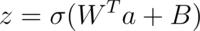
In the above expression:
Most of the computational workload in running neural networks comes from the convolution operation — which involves the multiplication of many floating point numbers. Large models with many weights have a very large number of convolution operations.
This computational cost could potentially be reduced by doing the multiplication in lower-precision integers instead of floating-point numbers. In an extreme case, as discussed in Understanding 1.58-bit Language Models, the 32-bit weights could potentially be represented by ternary numbers {-1, 0, +1} and the multiplication operations would be replaced by much simpler addition and subtraction operations. This is the intuition behind quantization.
The computational cost of digital arithmetic is quadratically related to the number of bits. As studied by Siddegowda et al in their paper on Neural Network Quantization (Section 2.1), using 8-bit integers instead of 32-bit floats leads to 16x higher performance, in terms of energy consumption. When there are billions of weights, the cost savings are very significant.
The quantizer function maps the high-precision (typically 32-bit floating point weights) to lower-precision integer weights.

The “knowledge” the model has acquired via training is represented by the value of its weights. When these weights are quantized to lower precision, a portion of their information is also lost. The challenge of quantization is to reduce the precision of the weights while maintaining the accuracy of the model.
One of the main reasons some quantization techniques are effective is that the relative values of the weights and the statistical properties of the weights are more important than their actual values. This is especially true for large models with millions or billions of weights. Later articles on quantized BERT models — BinaryBERT and BiBERT, on BitNet — which is a transformer LLM quantized down to binary weights, and on BitNet b1.58 — which quantizes transformers to use ternary weights, illustrate the use of successful quantization techniques. A Visual Guide to Quantization, by Maarten Grootendoorst, has many illustrations and graphic depictions of quantization.
Inference means using an AI model to generate predictions, such as the classification of an image, or the completion of a text string. When using a full-precision model, the entire data flow through the model is in 32-bit floating point numbers. When running inference through a quantized model, many parts — but not all, of the data flow are in lower precision.
The bias is typically not quantized because the number of bias terms is much less than the number of weights in a model. So, the cost savings is not enough to justify the overhead of quantization. The accumulator’s output is in high precision. The output of the activation is also in higher precision.
This article discussed the need to reduce the size of AI models and gave a high-level overview of ways to achieve reduced model sizes. It then introduced the basics of quantization, a method that is currently the most successful in reducing model sizes while managing to maintain an acceptable level of accuracy.
The goal of this series is to give you enough background to appreciate the extreme quantization of language models, starting from simpler models like BERT before finally discussing 1-bit LLMs and the recent work on 1.58-bit LLMs. To this end, the next few articles in this series present a semi-technical deep dive into the different subtopics like the mathematical operations behind quantization and the process of training quantized models. It is important to understand that because this is an active area of research and development, there are few standard procedures and different workers adopt innovative methods to achieve better results.
Reducing the Size of AI Models was originally published in Towards Data Science on Medium, where people are continuing the conversation by highlighting and responding to this story.
Originally appeared here:
Reducing the Size of AI Models

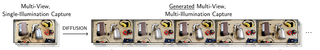
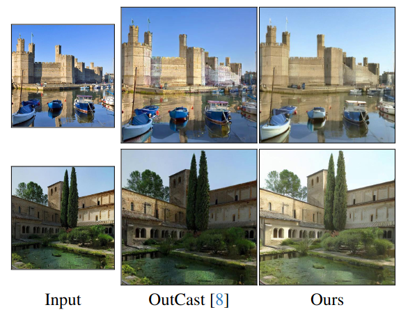
Relighting is the task of rendering a scene under a specified target lighting condition, given an input scene. This is a crucial task in computer vision and graphics. However, it is an ill-posed problem, because the appearance of an object in a scene results from a complex interplay between factors like the light source, the geometry, and the material properties of the surface. These interactions create ambiguities. For instance, given a photograph of a scene, is a dark spot on an object due to a shadow cast by lighting or is the material itself dark in color? Distinguishing between these factors is key to effective relighting.
In this blog post we discuss how different papers are tackling the problem of relighting via diffusion models. Relighting encompases a variety of subproblems including simple lighting adjustments, image harmonization, shadow removal and intrinsic decomposition. These areas are essential for refining scene edits such as balancing color and shadow across composited images or decoupling material and lighting properties. We will first introduce the problem of relighting and briefly discuss Diffusion models and ControlNets. We will then discuss different approaches that solve the problem of relighting in different types of scenes ranging from single objects to portraits to large scenes.
The goal is to decompose the scene into its fundamental components such as geometry, material, and light interactions and model them parametrically. Once solved then we can change it according to our preference. The appearance of a point in the scene can be described by the rendering equation as follows:
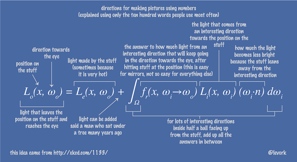
Most methods aim to solve for each single component of the rendering equation. Once solved, then we can perform relighting and material editing. Since the lighting term L is on both sides, this equation cannot be evaluated analytically and is either solved via Monte Carlo methods or approximation based approaches.
An alternate approach is data-driven learning, where instead of explicitly modeling the scene properties it directly learns from data. For example, instead of fitting a parametric function, a network can learn the material properties of the surface from data. Data-driven approaches have proven to be more powerful than parametric approaches. However they require a huge amount of high quality data which is really hard to collect especially for lighting and material estimation tasks.
Datasets for lighting and material estimation are rare as they require expensive, complex setups such as light stages to capture detailed lighting interactions. These setups are accessible to only a few organizations, limiting the availability of data for training and evaluation. There are no full-body ground truth light stage datasets publicly available which further highlights this challenge.
Computer vision has experienced a significant transformation with the advent of pre-training on vast amounts of image and video data available online. This has led to the development of foundation models, which serve as powerful general-purpose models that can be fine-tuned for a wide range of specific tasks. Diffusion models work by learning to model the underlying data distribution from independent samples, gradually reversing a noise-adding process to generate realistic data. By leveraging their ability to generate high-quality samples from learned distributions, diffusion models have become essential tools for solving a diverse set of generative tasks.
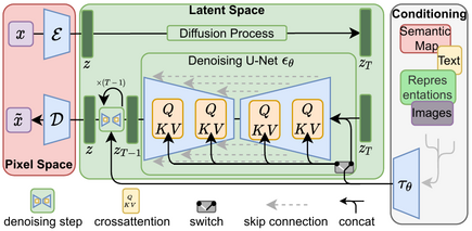
One of the most prominent examples of this is Stable Diffusion(SD), which was trained on the large-scale LAION-5B dataset that consists of 5 billion image text pairs. It has encoded a wealth of general knowledge about visual concepts making it suitable for fine-tuning for specific tasks. It has learnt fundamental relationships and associations during training such as chairs having 4 legs or recognizing structure of cars. This intrinsic understanding has allowed Stable Diffusion to generate highly coherent and realistic images and be used for fine tuning to predict other modalities. Based on this idea, the question arises if we can leverage pretrained SD to solve the problem of scene relighting.
So how do we fine-tune LDMs? A naive approach is to do transfer learning with LDMs. This would be freezing early layers (which capture general features) and fine tuning the model on the specific task. While this approach has been used by some papers such as Alchemist (for Material Transfer), it requires a large amount of paired data for the model to generalize well. Another drawback to this approach is the risk of catastrophic forgetting, where the model losses the knowledge gained during pretraining. This would limit its capability on generalizing across various conditions.
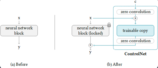
Another approach to fine-tuning such large models is by introducing a ControlNet. Here, a copy of the network is made and the weights of the original network are frozen. During training only the duplicate network weights are updated and the conditioning signal is passed as input to the duplicate network. The original network continues to leverage its pretrained knowledge.
While this increases the memory footprint, the advantage is that we dont lose the generalization capabilities acquired from training on large scale datasets. It ensures that it retains its ability to generate high-quality outputs across a wide range of prompts while learning the task specific relationships needed for the current task.
Additionally it helps the model learn robust and meaningful connections between control input and the desired output. By decoupling the control network from the core model, it avoids the risk of overfitting or catastrophic forgetting. It also needs significantly less paired data to train.
While there are other techniques for fine-tuning foundational models — such as LoRA (Low-Rank Adaptation) and others — we will focus on the two methods discussed: traditional transfer learning and ControlNet. These approaches are particularly relevant for understanding how various papers have tackled image-based relighting using diffusion models.
Introduction
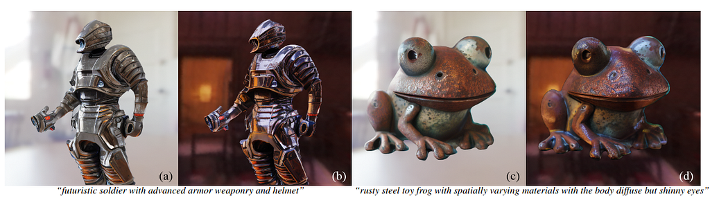
This work proposes fine grained control over relighting of an input image. The input image can either be generated or given as input. Further it can also change the material of the object based on the text prompt. The objective is to exert fine-grained control on the effects of lighting.
Method
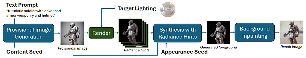
Given an input image, the following preprocessing steps are applied:
Once these images are generated, they train a ControlNet module. The input image and the mask are passed through an encoder decoder network which outputs a 12 channel feature map. This is then multiplied with the radiance cues images that are channel wise concatenated together. Thus during training, the noisy target image is denoised with this custom 12 channel image as conditioning signal.
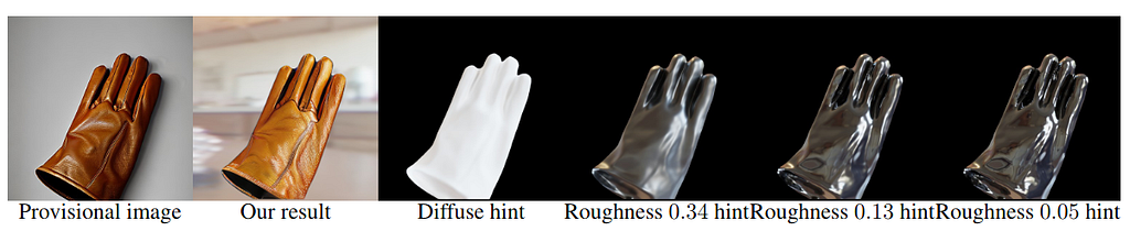
Additionally an appearance seed is provided to procure consistent appearance under different illumination. Without it the network renders a different interpretation of light-matter interaction. Additionally one can provide more cues via text to alter the appearance such as by adding “plastic/shiny metallic” to change the material of the generated image.
Implementation
The dataset was curated using 25K synthetic objects from Objaverse. Each object was rendered from 4 unique views and lit with 12 different lighting conditions ranging from point source lighting, multiple point source, environment maps and area lights. For training, the radiance cues were rendered in blender.
The ControlNet module uses stable diffusion v2.1 as base pretrained model to refine. Training took roughly 30 hours on 8x NVIDIA V100 GPUs. Training data was rendered in Blender at 512×512 resolution.
Results
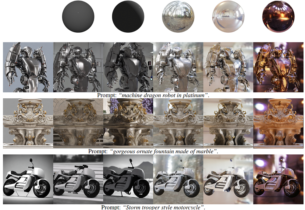
This figure shows the provisional image as reference and the corresponding target lighting under which the object is relit.
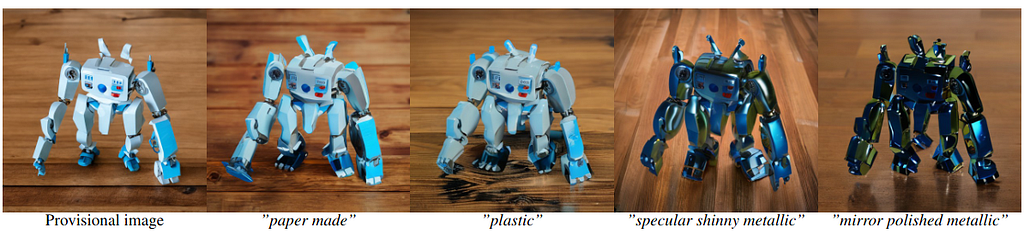
This figure shows how the text prompt can be used to change the material of the object.
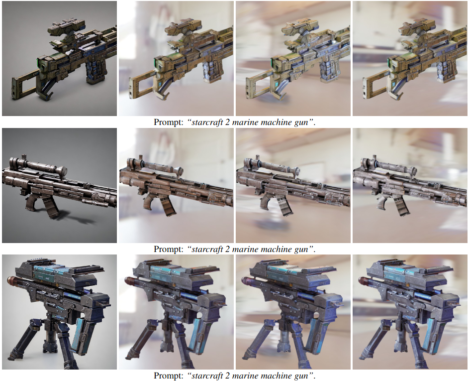
This figure shows more results of AI generated provisional images that are then rendered under different input environment light conditions.

This figure shows the different solutions the network comes up to resolve light interaction if the appearance seed is not fixed.
Limitations
Due to training on synthetic objects, the method is not very good with real images and works much better with AI generated provisional images. Additionally the material light interaction might not follow the intention of the prompt. Since it relies on depth maps for generating radiance cues, it may fail to get satisfactory results. Finally generating a rotating light video may not result in consistent results.
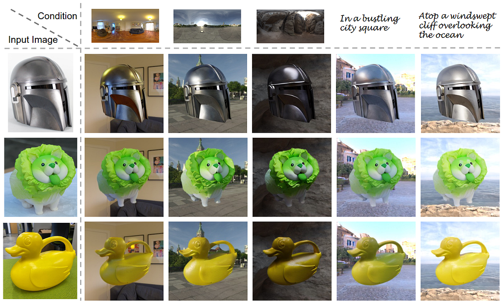
Introduction
This work proposes an end to end 2D relighting diffusion model. This model learns physical priors from synthetic dataset featuring physically based materials and HDR environment maps. It can be further used to relight multiple views and be used to create a 3D representation of the scene.
Method
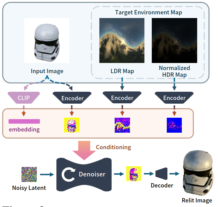
Given an image and a target HDR environment map, the goal is to learn a model that can synthesize a relit version of the image which here is a single object. This is achieved by adopting a pre-trained Zero-1-to-3 model. Zero-1-to-3 is a diffusion model that is conditioned on view direction to render novel views of an input image. They discard its novel view synthesis components. To incorporate lighting conditions, they concatenate input image and environment map encodings with the denoising latent.
The input HDR environment map E is split into two components: E_l, a tone-mapped LDR representation capturing lighting details in low-intensity regions, and E_h, a log-normalized map preserving information across the full spectrum. Together, these provide the network with a balanced representation of the energy spectrum, ensuring accurate relighting without the generated output appearing washed out due to extreme brightness.
Additionally the CLIP embedding of the input image is also passed as input. Thus the input to the model is the Input Image, LDR Image, Normalized HDR Image and CLIP embedding of Image all conditioning the denoising network. This network is then used as prior for further 3D object relighting.
Implementation
The model is trained on a custom Relit Objaverse Dataset that consists of 90K objects. For each object there are 204 images that are rendered under different lighting conditions and viewpoints. In total, the dataset consists of 18.4 M images at resolution 512×512.
The model is finetuned from Zero-1-to-3’s checkpoint and only the denoising network is finetined. The input environment map is downsampled to 256×256 resolution. The model is trained on 8 A6000 GPUs for 5 days. Further downstream tasks such as text-based relighting and object insertion can be achieved.
Results
They show comparisons with different backgrounds and comparisons with other works such as DilightNet and IC-Light.
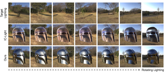
This figure compares the relighting results of their method with IC-Light, another ControlNet based method. Their method can produce consistent lighting and color with the rotating environment map.
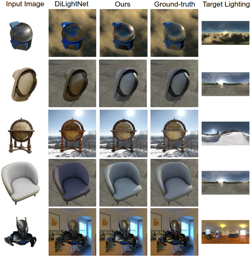
This figure compares the relighting results of their method with DiLightnet, another ControlNet based method. Their method can produce specular highlights and accurate colors.
Limitations
A major limitation is that it only produces low image resolution (256×256). Additionally it only works on objects and performs poorly for portrait relighting.

Introduction
Image Harmonization is the process of aligning the color and lighting features of the foreground subject with the background to make it a plausible composition. This work proposes a diffusion based approach to solve the task.
Method
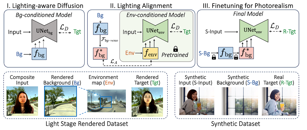
Given an input composite image, alpha mask and a target background, the goal is to predict a relit portrait image. This is achieved by training a ControlNet to predict the Harmonized image output.
In the first stage, we train a background control net model that takes the composite image and target background as input and outputs a relit portrait image. During training, the denoising network takes the noisy target image concatenated with composite image and predicts the noise. The background is provided as conditioning via the control net. Since background image by itself are LDR, they do not provide sufficient signals for relighting purposes.
In the second stage, an environment map control net model is trained. The HDR environment map provide lot more signals for relighting and this gives lot better results. However at test time, the users only provide LDR backgrounds. Thus, to bridge this gap, the 2 control net models are aligned with each other.
Finally more data is generated using the environment map ControlNet model and then the background ControlNet model is finetuned to generate more photo realistic results.
Implementation
The dataset used for training consists of 400k image pair samples that were curated using 100 lightstage. In the third stage additional 200k synthetic samples were generated for finetuning for photorealism.
The model is finetuned from InstructPix2PIx checkpoint The model is trained on 8 A100 GPUs at 512×512 resolution.
Results

This figure shows how the method neutralizes pronounced shadows in input which are usually hard to remove. On the left is input and right is relit image.
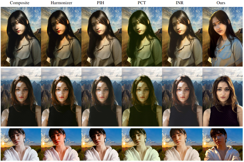
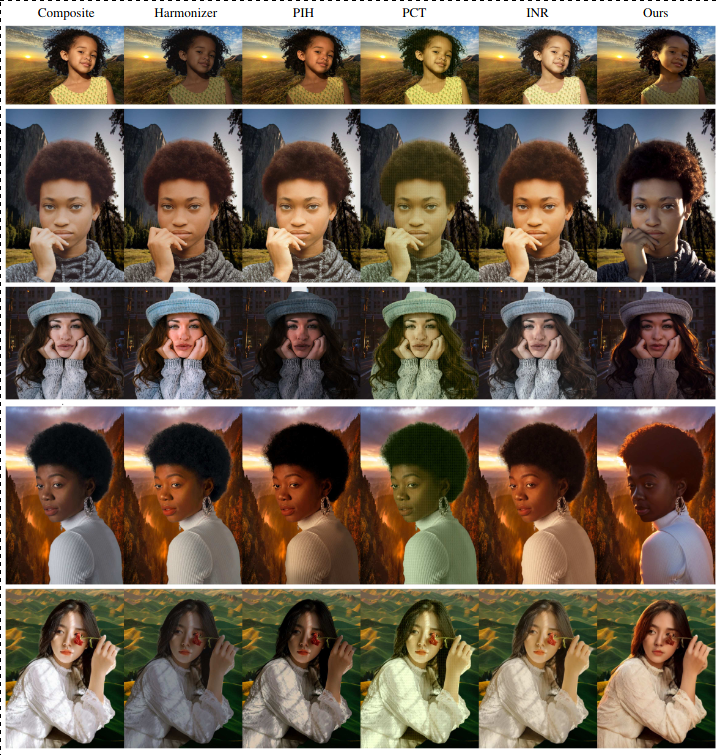
The figures show results on real world test subjects. Their method is able to remove shadows and make the composition more plausible compared to other methods.
Limitations
While this method is able to plausibly relight the subject, it is not great at identity preservation and struggles in maintaining color of the clothes or hair. Further it may struggle to eliminate shadow properly. Also it does not estimate albedo which is crucial for complex light interactions.
Introduction
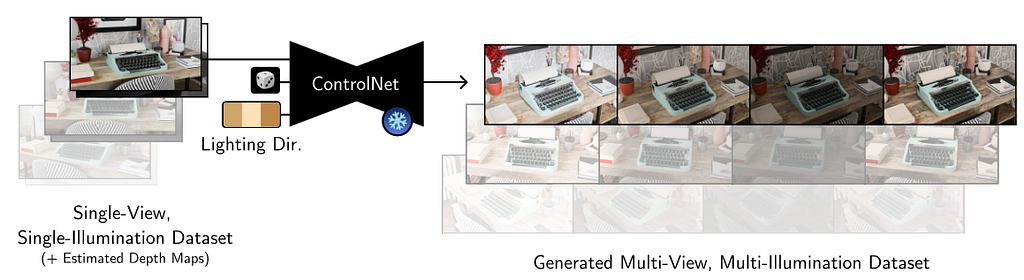
This work proposes a 2D relighting diffusion model that is further used to relight a radiance field of a scene. It first trains a ControlNet model to predict the scene under novel light directions. Then this model is used to generate more data which is eventually used to fit a relightable radiance field. We discuss the 2D relighting model in this section.
Method
Given a set of images X_i with corresponding depth map D (that is calculated via off the shelf methods), and light direction l_i the goal is to predict the scene under light direction l_j. During training, the input to the denoising network is X_i under random illumination, depth map D concatenated with noisy target image X_j. The light direction is encoded with 4th order SH and conditioned via ControlNet model.
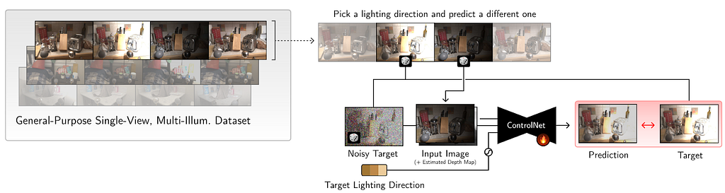
Although this leads to decent results, there are some significant problems. It is unable to preserve colors and leads to loss in contrast. Additionally it produces distorted edges. To resolve this, they color-match the predictions to input image to compensate for color difference. This is done by converting the image to LAB space and then channel normalization. The loss is then taken between ground-truth and denoised output. To preserve edges, the decoder was pretrained on image inpainting tasks which was useful in preserving edges. This network is then used to create corresponding scene under novel light directions which is further used to create a relightable radiance field representation.
Implementation
The method was developed upon Multi-Illumination dataset. It consists of 1000 real scenes of indoor scenes captured under 25 lighting directions. The images also consist of a diffuse and a metallic sphere ball that is useful for obtaining the light direction in world coordinates. Additionally some more scenes were rendered in Blender. The network was trained on images at resolution 1536×1024 and training consisted of 18 non-front facing light directions on 1015 indoor scenes.
The ControlNet module was trained using Stable Diffusion v2.1 model as backbone. It was trained on multiple A6000 GPUs for 150K iterations.
Results
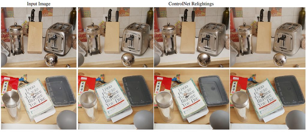
Here the diffuse spheres show the test time light directions. As can be seen, the method can render plausible relighting results
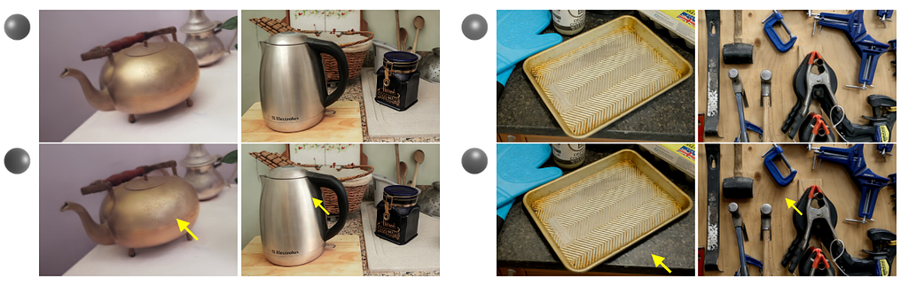
This figure shows how with the changing light direction, the specular highlights and shadows are moving as evident on the shiny highlight on the kettle.
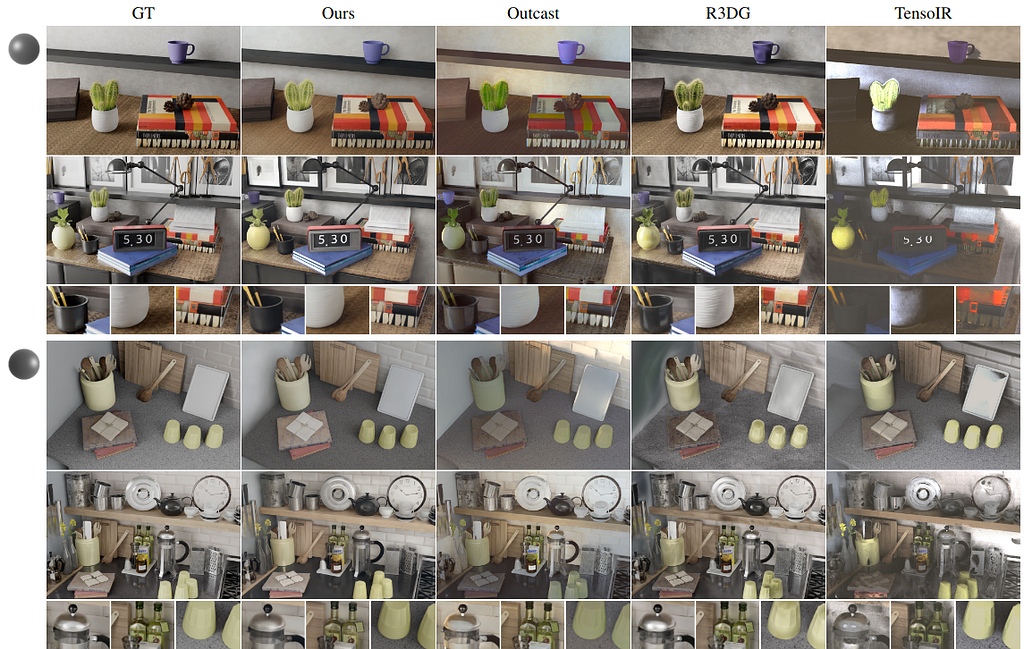
This figure compares results with other relightable radiance field methods. Their method clearly preserves color and contrast much better compared to other methods.
Limitations
The method does not enforce physical accuracy and can produce incorrect shadows. Additionally it also struggles to completely remove shadows in a fully accurate way. Also it does work reasonably for out of distribution scenes where the variance in lighting is not much.
Introduction
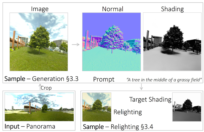
This work proposes a single view shading estimation method to generate a paired image and its corresponding direct light shading. This shading can then be used to guide the generation of the scene and relight a scene. They approach the problem as an intrinsic decomposition problem where the scene can be split into Reflectance and Shading. We will discuss the relighting component here.
Method
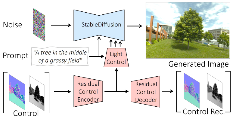
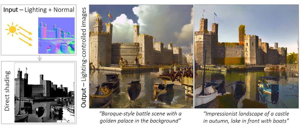
Given an input image, its corresponding surface normal, text conditioning and a target direct shading image, they generate a relit stylized image. This is achieved by training a ControlNet module.
During training, the noisy target image is passed to the denoising network along with text conditioning. The normal and target direct shading image are concatenated and passed through a Residual Control Encoder. The feature map is then used to condition the network. Additionally its also reconstructed back via Residual Control Decoder to regularize the training
Implementation
The dataset consists of Outdoor Laval Dataset which consist of outdoor real world HDR panoramas. From these images, 250 512×512 images are cropped and various camera effects are applied. The dataset consists of 51250 samples of LDR images and text prompts along with estimated normal and shading maps. The normals maps were estimated from depth maps that were estimated using off the shelf estimators.
The ControlNet module was finetuned from stable diffusion v1.5. The network was trained for two epochs. Other training details are not shared.
Results
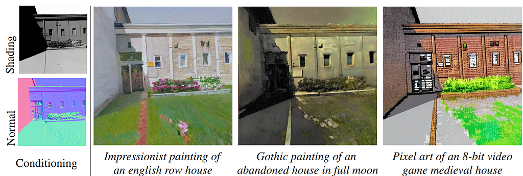
This figure shows that the generated images feature consistent lighting aligned with target shading for custom stylized text prompts. This is different from other papers discussed whose sole focus is on photorealism.
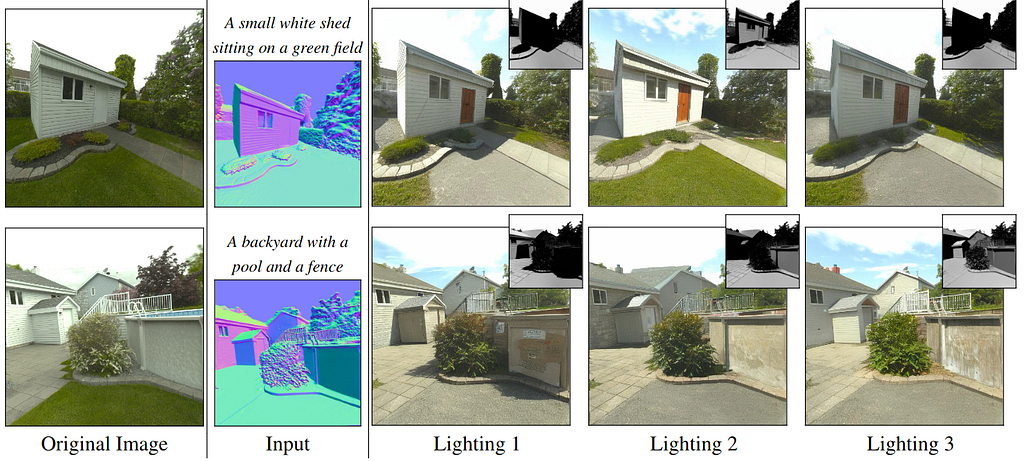
This figure shows identity preservation under different lighting conditions.
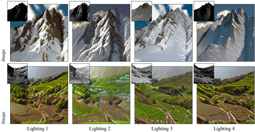
This figure shows results on different styles and scenes under changing lighting conditions.
This figure compares relighting with another method. Utilizing the diffusion prior helps with generalization and resolving shading disambiguation.
Limitations
Since this method assumes directional lighting, it enables tracing rays in arbitrary direction. It requires shading cues to generate images which are non trivial to obtain. Further their method does not work for portraits and indoor scenes.
We have discussed a non-exhaustive list of papers that leverage 2D diffusion models for relighting purposes. We explored different ways to condition Diffusion models for relighting ranging from radiance cues, direct shading images, light directions and environment maps. Most of these methods show results on synthetic datasets and dont generalize well to out of distribution datasets. There are more papers coming everyday and the base models are also improving. Recently IC-Light2 was released which is a ControlNet model based upon Flux models. It will be interesting which direction it takes as maintaining identities is tricky.
References:
Let There Be Light! Diffusion Models and the Future of Relighting was originally published in Towards Data Science on Medium, where people are continuing the conversation by highlighting and responding to this story.
Originally appeared here:
Let There Be Light! Diffusion Models and the Future of Relighting
Go Here to Read this Fast! Let There Be Light! Diffusion Models and the Future of Relighting


Offline Reinforcement Learning and Simulation To Strategize Online Engagement
Originally appeared here:
Using Offline Reinforcement Learning To Trial Online Platform Interventions

In this position paper, I discuss the premise that a lot of potential performance enhancement is left on the table because we don’t often address the potential of dynamic execution.
I guess I need to first define what is dynamic execution in this context. As many of you are no doubt aware of, we often address performance optimizations by taking a good look at the model itself and what can be done to make processing of this model more efficient (which can be measured in terms of lower latency, higher throughput and/or energy savings).
These methods often address the size of the model, so we look for ways to compress the model. If the model is smaller, then memory footprint and bandwidth requirements are improved. Some methods also address sparsity within the model, thus avoiding inconsequential calculations.
Still… we are only looking at the model itself.
This is definitely something we want to do, but are there additional opportunities we can leverage to boost performance even more? Often, we overlook the most human-intuitive methods that don’t focus on the model size.
Hard vs Easy
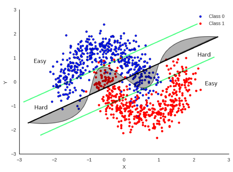
In Figure 1, there’s a simple example (perhaps a bit simplistic) regarding how to classify between red and blue data points. It would be really useful to be able to draw a decision boundary so that we know the red and blue points are on opposite sides of the boundary as much as possible. One method is to do a linear regression whereby we fit a straight line as best as we can to separate the data points as much as possible. The bold black line in Figure 1 represents one potential boundary. Focusing only on the bold black line, you can see that there is a substantial number of points that fall on the wrong side of the boundary, but it does a decent job most of the time.
If we focus on the curved line, this does a much better job, but it’s also more difficult to compute as it’s no longer a simple, linear equation. If we want more accuracy, clearly the curve is a much better decision boundary than the black line.
But let’s not just throw out the black line just yet. Now let’s look at the green parallel lines on each side of the black boundary. Note that the linear decision boundary is very accurate for points outside of the green line. Let’s call these points “Easy”.
In fact, it is 100% as accurate as the curved boundary for Easy points. Points that lie inside the green lines are “Hard” and there is a clear advantage to using the more complex decision boundary for these points.
So… if we can tell if the input data is hard or easy, we can apply different methods to solving the problem with no loss of accuracy and a clear savings of computations for the easy points.
This is very intuitive as this is exactly how humans address problems. If we perceive a problem as easy, we often don’t think too hard about it and give an answer quickly. If we perceive a problem as being hard, we think more about it and often it takes more time to get to the answer.
So, can we apply a similar approach to AI?
Dynamic Execution Methods
In the dynamic execution scenario, we employ a set of specialized techniques designed to scrutinize the specific query at hand. These techniques involve a thorough examination of the query’s structure, content, and context with the aim of discerning whether the problem it represents can be addressed in a more straightforward manner.
This approach mirrors the way humans tackle problem-solving. Just as we, as humans, are often able to identify problems that are ’easy’ or ’simple’ and solve them with less effort compared to ’hard’ or ’complex’ problems, these techniques strive to do the same. They are designed to recognize simpler problems and solve them more efficiently, thereby saving computational resources and time.
This is why we refer to these techniques as Dynamic Execution. The term ’dynamic’ signifies the adaptability and flexibility of this approach. Unlike static methods that rigidly adhere to a predetermined path regardless of the problem’s nature, Dynamic Execution adjusts its strategy based on the specific problem it encounters, that is, the opportunity is data dependent.
The goal of Dynamic Execution is not to optimize the model itself, but to optimize the compute flow. In other words, it seeks to streamline the process through which the model interacts with the data. By tailoring the compute flow to the data presented to the model, Dynamic Execution ensures that the model’s computational resources are utilized in the most efficient manner possible.
In essence, Dynamic Execution is about making the problem-solving process as efficient and effective as possible by adapting the strategy to the problem at hand, much like how humans approach problem-solving. It is about working smarter, not harder. This approach not only saves computational resources but also improves the speed and accuracy of the problem-solving process.
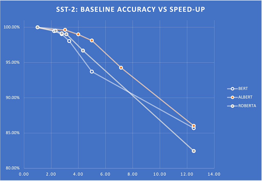
Early Exit
This technique involves adding exits at various stages in a deep neural network (DNN). The idea is to allow the network to terminate the inference process earlier for simpler tasks, thus saving computational resources. It takes advantage of the observation that some test examples can be easier to predict than others [1], [2].
Below is an example of the Early Exit strategy in several encoder models, including BERT, ROBERTA, and ALBERT.
We measured the speed-ups on glue scores for various entropy thresholds. Figure 2 shows a plot of these scores and how they drop with respect to the entropy threshold. The scores show the percentage of the baseline score (that is, without Early Exit). Note that we can get 2x to 4X speed-up without sacrificing much quality.
Speculative Sampling
This method aims to speed up the inference process by computing several candidate tokens from a smaller draft model. These candidate tokens are then evaluated in parallel in the full target model [3], [4].
Speculative sampling is a technique designed to accelerate the decoding process of large language models [5], [6]. The concept behind speculative sampling is based on the observation that the latency of parallel scoring of short continuations, generated by a faster but less powerful draft model, is comparable to that of sampling a single token from the larger target model. This approach allows multiple tokens to be generated from each transformer call, increasing the speed of the decoding process.
The process of speculative sampling involves two models: a smaller, faster draft model and a larger, slower target model. The draft model speculates what the output is several steps into the future, while the target model determines how many of those tokens we should accept. The draft model decodes several tokens in a regular autoregressive fashion, and the probability outputs of the target and the draft models on the new predicted sequence are compared. Based on some rejection criteria, it is determined how many of the speculated tokens we want to keep. If a token is rejected, it is resampled using a combination of the two distributions, and no more tokens are accepted. If all speculated tokens are accepted, an additional final token can be sampled from the target model probability output.
In terms of performance boost, speculative sampling has shown significant improvements. For instance, it was benchmarked with Chinchilla, a 70 billion parameter language model, achieving a 2–2.5x decoding speedup in a distributed setup, without compromising the sample quality or making modifications to the model itself. Another example is the application of speculative decoding to Whisper, a general purpose speech transcription model, which resulted in a 2x speed-up in inference throughput [7], [8]. Note that speculative sampling can be used to boost CPU inference performance, but the boost will likely be less (typically around 1.5x).
In conclusion, speculative sampling is a promising technique that leverages the strengths of both a draft and a target model to accelerate the decoding process of large language models. It offers a significant performance boost, making it a valuable tool in the field of natural language processing. However, it is important to note that the actual performance boost can vary depending on the specific models and setup used.
StepSaver
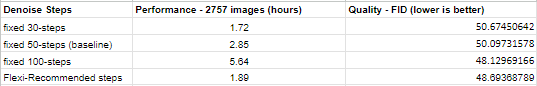
This is a method that could also be called Early Stopping for Diffusion Generation, using an innovative NLP model specifically fine-tuned to determine the minimal number of denoising steps required for any given text prompt. This advanced model serves as a real-time tool that recommends the ideal number of denoising steps for generating high-quality images efficiently. It is designed to work seamlessly with the Diffusion model, ensuring that images are produced with superior quality in the shortest possible time. [9]
Diffusion models iteratively enhance a random noise signal until it closely resembles the target data distribution [10]. When generating visual content such as images or videos, diffusion models have demonstrated significant realism [11]. For example, video diffusion models and SinFusion represent instances of diffusion models utilized in video synthesis [12][13]. More recently, there has been growing attention towards models like OpenAI’s Sora; however, this model is currently not publicly available due to its proprietary nature.
Performance in diffusion models involves a large number of iterations to recover images or videos from Gaussian noise [14]. This process is called denoising and is trained on a specific number of iterations of denoising. The number of iterations in this sampling procedure is a key factor in the quality of the generated data, as measured by metrics, such as FID.
Latent space diffusion inference uses iterations in feature space, and performance suffers from the expense of many iterations required for quality output. Various techniques, such as patching transformation and transformer-based diffusion models [15], improve the efficiency of each iteration.
StepSaver dynamically recommends significantly lower denoising steps, which is critical to address the slow sampling issue of stable diffusion models during image generation [9]. The recommended steps also ensure better image quality. Figure 3 shows that images generated using dynamic steps result in a 3X throughput improvement and a similar image quality compared to static 100 steps.
LLM Routing
Dynamic Execution isn’t limited to just optimizing a specific task (e.g. generating a sequence of text). We can take a step above the LLM and look at the entire pipeline. Suppose we are running a huge LLM in our data center (or we’re being billed by OpenAI for token generation via their API), can we optimize the calls to LLM so that we select the best LLM for the job (and “best” could be a function of token generation cost). Complicated prompts might require a more expensive LLM, but many prompts can be handled with much lower cost on a simpler LLM (or even locally on your notebook). So if we can route our prompt to the appropriate destination, then we can optimize our tasks based on several criteria.
Routing is a form of classification in which the prompt is used to determine the best model. The prompt is then routed to this model. By best, we can use different criteria to determine the most effective model in terms of cost and accuracy. In many ways, routing is a form of dynamic execution done at the pipeline level where many of the other optimizations we are focusing on in this paper is done to make each LLM more efficient. For example, RouteLLM is an open-source framework for serving LLM routers and provides several mechanisms for reference, such as matrix factorization. [16] In this study, the researchers at LMSys were able to save 85% of costs while still keeping 95% accuracy.
Conclusion
This certainly was not meant to be an exhaustive study of all dynamic execution methods, but it should provide data scientists and engineers with the motivation to find additional performance boosts and cost savings from the characteristics of the data and not solely focus on model-based methods. Dynamic Execution provides this opportunity and does not interfere with or hamper traditional model-based optimization efforts.
Unless otherwise noted, all images are by the author.
[1] K. Liao, Y. Zhang, X. Ren, Q. Su, X. Sun, and B. He, “A Global Past-Future Early Exit Method for Accelerating Inference of Pre-trained Language Models,” in Conference of the North American Chapter of the Association for Computational Linguistics: Human Language Technologies, pp. 2013–2023, Association for Computational Linguistics (ACL), June 2021.
[2] F. Ilhan, K.-H. Chow, S. Hu, T. Huang, S. Tekin, W. Wei, Y. Wu, M. Lee, R. Kompella, H. Latapie, G. Liu, and L. Liu, “Adaptive Deep Neural Network Inference Optimization with EENet,” Dec. 2023. arXiv:2301.07099 [cs].
[3] Y. Leviathan, M. Kalman, and Y. Matias, “Fast Inference from Transformers via Speculative Decoding,” May 2023. arXiv:2211.17192 [cs].
[4] H. Barad, E. Aidova, and Y. Gorbachev, “Leveraging Speculative Sampling and KV-Cache Optimizations Together for Generative AI using OpenVINO,” Nov. 2023. arXiv:2311.04951 [cs].
[5] C. Chen, S. Borgeaud, G. Irving, J.-B. Lespiau, L. Sifre, and J. Jumper, “Accelerating Large Language Model Decoding with Speculative Sampling,” Feb. 2023. arXiv:2302.01318 [cs] version: 1.
[6] J. Mody, “Speculative Sampling,” Feb. 2023.
[7] J. Gante, “Assisted Generation: a new direction toward low-latency text generation,” May 2023.
[8] S. Gandhi, “Speculative Decoding for 2x Faster Whisper Inference.”
[9] J. Yu and H. Barad, “Step Saver: Predicting Minimum Denoising Steps for Diffusion Model Image Generation,” Aug. 2024. arXiv:2408.02054 [cs].
[10] Notomoro, “Diffusion Model: A Comprehensive Guide With Example,” Feb. 2024. Section: Artificial Intelligence.
[11] T. H¨oppe, A. Mehrjou, S. Bauer, D. Nielsen, and A. Dittadi, “Diffusion Models for Video Prediction and Infilling,” Nov. 2022. arXiv:2206.07696 [cs, stat].
[12] J. Ho, T. Salimans, A. Gritsenko, W. Chan, M. Norouzi, and D. J. Fleet, “Video Diffusion Models,” June 2022. arXiv:2204.03458 [cs].
[13] Y. Nikankin, N. Haim, and M. Irani, “SinFusion: Training Diffusion Models on a Single Image or Video,” June 2023. arXiv:2211.11743 [cs].
[14] Z. Chen, Y. Zhang, D. Liu, B. Xia, J. Gu, L. Kong, and X. Yuan, “Hierarchical Integration Diffusion Model for Realistic Image Deblurring,” Sept. 2023. arXiv:2305.12966 [cs]
[15] W. Peebles and S. Xie, “Scalable Diffusion Models with Transformers,” Mar. 2023. arXiv:2212.09748 [cs].
[16] I. Ong, A. Almahairi, V. Wu, W.-L. Chiang, T. Wu, J. E. Gonzalez, M. W. Kadous, and I. Stoica, “RouteLLM: Learning to Route LLMs with Preference Data,” July 2024. arXiv:2406.18665 [cs].
Dynamic Execution was originally published in Towards Data Science on Medium, where people are continuing the conversation by highlighting and responding to this story.
Originally appeared here:
Dynamic Execution
Tips and tricks for teachers and mentors about teaching tech
Originally appeared here:
What I Learned from Teaching Tech for the Past 2 Years
Go Here to Read this Fast! What I Learned from Teaching Tech for the Past 2 Years


It was a beautiful spring day in New York City. The skies were clear, and temperatures were climbing toward 20 degrees Celsius. The Yankees prepared to play the Kansas City Royals at Yankee Stadium, and the Rangers were facing off against the Devils at Madison Square Garden. Nothing seemed out of the ordinary, yet the people gathering at the Equitable Center in Midtown Manhattan were about to experience something truly unique. They were about to witness the historic event when a computer, for the first time, would beat a reigning world champion in chess under standard tournament conditions.
Representing humans was Gary Kasparov, widely recognized as the world’s top chess player at the time. And representing the machines, Deep Blue — a chess computer developed by IBM. Going into the final and 6th game of the match, both players had 2.5 points. It was today that the winner was to be decided.
Gary started out as black, but made an early error and faced a strong, aggressive attack from Deep Blue. After just 19 moves it was all over. Kasparov, feeling demoralized and under pressure, resigned, believing his position was untenable. A symbolic, and by many hailed as one of the most important moments between man and machine was a fact. This landmark event marked a turning point in AI development, highlighting the potential — and challenges — of strategic AI.

Inspired by the recent advancements in generative AI — and my own experiments with large language models and their strategic capabilities — I have increasingly been thinking about strategic AI. How have we tried to approach this topic in the past? What are the challenges and what remains to be solved before we have a more generalist strategic AI agent?
As data scientists, we are increasingly implementing AI solutions for our clients and employers. For society at large, the ever-increasing interaction with AI makes it critical to understand the development of AI and especially strategic AI. Once we have autonomous agents with the ability to maneuver well in strategic contexts, this will have profound implications for everyone.
But what exactly do we mean when we say strategic AI? At its core, strategic AI involves machines making decisions that not only consider potential actions, but also anticipate and influence the responses of others. It’s about maximizing expected outcomes in complex, uncertain environments.
In this article, we’ll define strategic AI, explore what it is and how it has developed through the years since IBM’s Deep Blue beat Kasparov in 1997. We will try to understand the general architecture of some of the models, and in addition also examine how large language models (LLMs) fit into the picture. By understanding these trends and developments, we can better prepare for a world where autonomous AI agents are integrated into society.

A deeper discussion around strategic AI starts with a well-formulated definition of the topic.
When we consider strategy in a commercial setting, we often tend to associate it with topics like long-term thinking, resource allocation and optimization, a holistic understanding of inter-dependences in an organization, alignment of decisions with the purpose and mission of the company and so on. While these topics are useful to consider, I often prefer a more game theoretical definition of strategy when dealing with AI and autonomous agents. In this case we define being strategic as:
Choosing a course of action that maximizes your expected payoff by considering not just your own potential actions but also how others will respond to those actions and how your decisions impact the overall dynamics of the environment.
The critical part of this definition is that strategic choices are choices that do not occur in a vacuum, but rather in the context of other participants, be they humans, organizations or other AIs. These other entities can have similar or conflicting goals of their own and may also try to act strategically to further their own interests.
Also, strategic choices always seek to maximize expected payoffs, whether those payoffs are in terms of money, utility, or other measures of value. If we wanted to incorporate the more traditional “commercial” topics related to strategy we could imagine that we want to maximize the value of a company 10 years from now. In this case, to formulate a good strategy we would need to take a “long term” view, and might also consider the “purpose and mission” of the company as well, to ensure alignment with the strategy. However, pursuing these exercises are merely a consequence of what it actually means to act strategically.
The game-theoretic view of strategy captures the essence of strategic decision-making and consequently lets us clearly define what we mean by strategic AI. From the definition we see that if an AI system or agent is to act strategically, it needs to have a few core capabilities. Specifically, it will need to be able to:
There is currently no well-known, or well published system, that is capable of all of these actions in an autonomous way in the real world. However, given the recent advances in AI systems and the rapid rise of LLMs that might be about to change!

Before we proceed with further discussion into strategic AI, it might be useful to review some concepts and ideas from game theory. A lot of the work that has been done around strategic AI has a foundation in game theoretic concepts and using theorems from game theory can show the existence of certain properties that make some games and situations easier to deal with than others. It also helps to highlight some of the shortcomings of game theory when it comes to real world situations and highlights where we might be better off looking in other directions for inspiration.
We define a game as a mathematical model comprising three key components:
This formal structure allows for the systematic study of strategic interactions and decision-making processes.
When speaking on games it also makes sense to look at the distinction between finite and infinite games.
Finite games have a fixed set of players, defined rules, and a clear endpoint. The objective is to win, and examples include chess, go, checkers, and most traditional board games.
Infinite games on the other hand have no predetermined endpoint, and the rules can evolve over time. The objective is not to win but to continue playing. Real-world scenarios like business competition or societal evolution can be viewed as infinite games. The Cold War can be viewed as an example of an infinite game. It was a prolonged geopolitical struggle between the United States and its allies (the West) and the Soviet Union and its allies (the East). The conflict had no fixed endpoint, and the strategies and “rules” evolved over time.
Sometimes we might be able to find smaller games within a larger game context. Mathematically, subgames are self-contained games in their own right, and the need to satisfy a few different criteria:
We can visualize a subgame if we imagine a large tree representing an entire game. A subgame is like selecting a branch of this tree starting from a certain point (node) and including everything that extends from it, while also ensuring that any uncertainties are fully represented within this branch.
The core idea behind a subgame makes it useful for our discussion around strategic AI. The reason is primarily that some infinite games between players might be very complex and difficult to model while if we choose to look at smaller games within that game, we can have more success applying game theoretical analysis.
Coming back to our example with the Cold War as an infinite game, we can recognize several subgames within that context. Some examples include:
The Cuban Missile Crisis (1962):
The Berlin Blockade and Airlift (1948–1949):
Although of course very difficult and complex to deal with, both “subgames” are easier to analyze and develop responses to than to the whole of the Cold War. They had a defined set of players, with a limited set of strategies and payoffs, and also a clearer time frame. This made them both more applicable for game theoretical analysis.
In the context of strategic AI, analyzing these sub-games is crucial for developing intelligent systems capable of making optimal decisions in complex, dynamic environments.
Two player games are simply a game between two players. This could for example be a game between two chess players, or coming back to our Cold War example, the West vs the East. Having only two players in the game simplifies the analysis but still captures essential competitive or cooperative dynamics. Many of the results in game theory are based around two player games.
Zero-sum games are a subset of games where one player’s gain is another player’s loss. The total payoff remains constant, and the players are in direct competition.
A Nash Equilibrium (NE) is a set of strategies where no player can gain additional benefit by unilaterally changing their own strategy, assuming the other players keep theirs unchanged. In this state, each player’s strategy is the best response to the strategies of the others, leading to a stable outcome where no player has an incentive to deviate.
For example, in the game Rock-Paper-Scissor (RPS), the NE is the state where all players play rock, paper and scissors, randomly, each with equal probability. If you as a player choose to play the NE strategy, you ensure that no other player can exploit your play and in a two player zero-sum games it can be shown that you will not lose in expectation, and that the worst you can do is break even.
However, playing a NE strategy might not always be the optimal strategy, especially if your opponent is playing in a predictably sub-optimal way. Consider a scenario with two players, A and B. If player B starts playing paper more, player A could recognize this and increase its frequency of playing scissors. However, this deviation from A could again be exploited by B again which could change and play more rock.
Reviewing the game theoretic concepts, it would seem the idea of a subgame is especially useful for strategic AI. The ability to find possible smaller and easier to analyze games within a larger context makes it easier to apply already know solutions and solvers.
For example, let’s say you are working on developing your career, something which could be classified as an infinite game and difficult to “solve”, but suddenly you get the opportunity to negotiate a new contract. This negotiation process presents an opportunity for a subgame within your career and would be much more approachable for a strategic AI using game theoretic concepts.
Indeed, humans have been creating subgames within our lives for thousands of years. About 1500 years ago in India, we created the origins of what is now known as chess. Chess turned out to be quite a challenge for AI to beat, but also allowed us to start developing more mature tools and techniques that could be used for even more complicated and difficult strategic situations.

Games have provided an amazing proving ground for developing strategic AI. The closed nature of games makes it easier to train models and develop solution techniques than in open ended systems. Games are clearly defined; the players are known and so are the payoffs. One of the biggest and earliest milestones was Deep Blue, the machine that beat the world champion in chess.
Deep Blue was a chess-playing supercomputer developed by IBM in the 1990s. As stated in the prologue, it made history in May 1997 by defeating the reigning world chess champion, Garry Kasparov, in a six-game match. Deep Blue utilized specialized hardware and algorithms capable of evaluating 200 million chess positions per second. It combined brute-force search techniques with heuristic evaluation functions, enabling it to search deeper into potential move sequences than any previous system. What made Deep Blue special was its ability to process vast numbers of positions quickly, effectively handling the combinatorial complexity of chess and marking a significant milestone in artificial intelligence.
However, as Gary Kasparov notes in his interview with Lex Fridman¹, Deep Blue was more of a brute force machine than anything else, so it’s perhaps hard to qualify it as any type of intelligence. The core of the search is basically just trial and error. And speaking of errors, it makes significantly less errors than humans, and according to Kasparov this is one of the features which made it hard to beat.
19 years after the Deep Blue victory in chess, a team from Google’s DeepMind produced another model that would contribute to a special moment in the history of AI. In 2016, AlphaGo became the first AI model to defeat a world champion go player, Lee Sedol.
Go is a very old board game with origins in Asia, known for its deep complexity and vast number of possible positions, far exceeding those in chess. AlphaGo combined deep neural networks with Monte Carlo tree search, allowing it to evaluate positions and plan moves effectively. The more time AlphaGo was given at inference, the better it performs.
The AI trained on a dataset of human expert games and improved further through self-play. What made AlphaGo special was its ability to handle the complexity of Go, utilizing advanced machine learning techniques to achieve superhuman performance in a domain previously thought to be resistant to AI mastery.
One could argue AlphaGo exhibits more intelligence than Deep Blue, given its exceptional ability to deeply evaluate board states and select moves. Move 37 from its 2016 game against Lee Sedol is a classic example. For those acquainted with Go, it was a shoulder hit at the fifth line and initially baffled commentators, including Lee Sedol himself. But as would later become clear, the move was a brilliant play and showcased how AlphaGo would explore strategies that human players might overlook and disregard.
One year later, Google DeepMind made headlines again. This time, they took many of the learnings from AlphaGo and created AlphaZero, which was more of a general-purpose AI system that mastered chess, as well as Go and shogi. The researchers were able to build the AI solely through self-play and reinforcement learning without prior human knowledge or data. Unlike traditional chess engines that rely on handcrafted evaluation functions and extensive opening libraries, AlphaZero used deep neural networks and a novel algorithm combining Monte Carlo tree search with self-learning.
The system started with only the basic rules and learned optimal strategies by playing millions of games against itself. What made AlphaZero special was its ability to discover creative and efficient strategies, showcasing a new paradigm in AI that leverages self-learning over human-engineered knowledge.
Continuing its domination in the AI space, the Google DeepMind team changed its focus to a highly popular computer game, StarCraft II. In 2019 they developed an AI called AlphaStar² which was able to achieve Grandmaster level play and rank higher than 99.8% of human players on the competitive leaderboard.
StarCraft II is a real time strategy game that provided several novel challenges for the team at DeepMind. The goal of the game is to conquer the opposing player or players, by gathering resources, constructing buildings and amassing armies that can defeat the opponent. The main challenges in this game arise from the enormous action space that needs to be considered, the real-time decision making, partial observability due to fog of war and the need for long-term strategic planning, as some games can last for hours.
By building on some of the techniques developed for previous AIs, like reinforcement learning through self-play and deep neural networks, the team was able to make a unique game engine. Firstly, they trained a neural net using supervised learning and human play. Then, they used that to seed another algorithm that could play against itself in a multi-agent game framework. The DeepMind team created a virtual league where the agents could explore strategies against each other and where the dominant strategies would be rewarded. Ultimately, they combined the strategies from the league into a super strategy that could be effective against many different opponents and strategies. In their own words³:
The final AlphaStar agent consists of the components of the Nash distribution of the league — in other words, the most effective mixture of strategies that have been discovered — that run on a single desktop GPU.
I love playing poker, and when I was living and studying in Trondheim, we used to have a weekly cash game which could get quite intense! One of the last milestones to be eclipsed by strategic AI was in the game of poker. Specifically, in one of the most popular forms of poker, 6-player no-limit Texas hold’em. In this game we use a regular deck of cards with 52 cards, and the play follows the following structure:
The players can use the cards on the table and the two cards on their hand to assemble a 5-card poker hand. For each round of the game, the players take turns placing bets, and the game can end at any of the rounds if one player places a bet that no one else is willing to call.
Though reasonably simple to learn, one only needs to know the hierarchy of the various poker hands, this game proved to be very difficult to solve with AI, despite ongoing efforts for several decades.
There are multiple factors contributing to the difficulty of solving poker. Firstly, we have the issue of hidden information, because you don’t know which cards the other players have. Secondly, we have a multiplayer setup with many players, with each extra player increasing the number of possible interactions and strategies exponentially. Thirdly, we have the no-limit betting rules, which allow for a complex betting structure where one player can suddenly decide to bet his entire stack. Fourth, we have an enormous game tree complexity due to the combinations of hole cards, community cards, and betting sequences. In addition, we also have complexity due to the stochastic nature of the cards, the potential for bluffing and the opponent modelling!
It was only in 2019 that a couple of researchers, Noam Brown and Tuomas Sandholm, finally cracked the code. In a paper published in Science, they describe a novel poker AI — Pluribus — that managed to beat the best players in the world in 6-player no-limit Texas hold’em.⁴ They conducted two different experiments, each consisting of a 10000 poker hands, and both experiments clearly showed the dominance of Pluribus.
In the first experiment, Pluribus played against 5 human opponents, achieving an average win rate of 48 mbb/game, with a standard deviation of 25 mbb/game. (mbb/game stands for milli big blind per game, how many big blinds is won per 1000 games played.) 48 mbb/game is considered a very high win rate, especially among elite poker players, and implies that Pluribus is stronger than the human opponents.
In the second experiment, the researchers had 5 versions of Pluribus play against 1 human. They set up the experiment so that 2 different humans would each play 5000 hands each against the 5 machines. Pluribus ended up beating the humans by an average of 32 mbb/game with a standard error of 15 mbb/game, again showing its strategic superiority.
The dominance of Pluribus is quite amazing, especially given all the complexities the researchers had to overcome. Brown and Sandholm came up with several smart strategies that helped Pluribus to become superhuman and computationally much more efficient than previous top poker AIs. Some of their techniques include:
There are quite a few interesting observations to draw from Pluribus, but perhaps the most interesting is that it doesn’t vary its play against different opponents, but instead has developed a robust strategy that is effective against a wide variety of players. Since a lot of poker players think they have to adjust their play to various situations and people, Pluribus shows us that this is not needed and probably not even optimal, given how it beat all the humans it played against.
In our short foray into game theory, we noted that if you play the NE strategy in two-player zero-sum games you are guaranteed not to lose in expectation. However, for a multiplayer game like 6-player poker there is no such guarantee. Noam Brown speculates⁵ that it is perhaps the adversarial nature of a game like poker which still makes it suitable to try to approach it with a NE strategy. Conversely, in a game like Risk where players can cooperate more, pursuing a NE strategy is not guaranteed to work, because, if you are playing a risk game with 6 people, there is nothing you can do if your 5 opponents decide to gang up on you and kill you.
Summarizing the history of strategic AI in games, we see a clear trend emerging. The games are slowly but surely becoming closer to the real-world strategic situations that humans find themselves in on an everyday basis.
Firstly, we are moving from a two-player to a multiplayer setting. This can be seen from the initial success in two-player games to multiplayer games like 6-player poker. Secondly, we are seeing an increase in the mastery of games with hidden information. Thirdly we are also seeing an increase in mastery of games with more stochastic elements.
Hidden information, multiplayer settings and stochastic events are the norm rather than the exception in strategic interactions among humans, so mastering these complexities is key in achieving a more general superhuman strategic AI that can navigate in the real world.

I recently ran an experiment where I let LLMs play the boardgame Risk against each other. My objective with the experiment was to gauge how well the LLMs could perform in a strategic setting, more of less out of the box. Quite a lot of detailed prompting were given to the agents to provide the right context, however, and perhaps not surprisingly, the LLM performance was rather mediocre.
You can find an article about the experiment here:
Exploring the Strategic Capabilities of LLMs in a Risk Game Setting
Summarizing some of the key findings from the experiment, the current generation of LLMs struggles with basic strategic concepts like fortification and recognizing winning moves. They also fail to eliminate other players when it would have been strategically beneficial for them to do so.
The above experiment indicates that even though we have seen a rapid improvement in the LLMs, they still lack the sophistication for strategic reasoning. Given their very general training data and how they have been constructed this shouldn’t come as a surprise.
So how do they fit into the discussion around strategic AI? To understand that, we need to understand what the LLMs really excel at. Perhaps the most promising feature of the LLMs is their ability to digest and generate vast amounts of text. And now with multimodal models, video and audio too. In other words, LLMs are great for interacting with the real world, both in human and other contexts. Recently, an AI team at Meta was able to combine the general language capabilities of a language model with the strategic insights of a strategy engine.
The game of Diplomacy is a 2 to 7-player strategy game, which Meta describes as a mix between Risk, Poker and the TV show Survivor. The players start out with a map of Europe ca. 1900, and the objective is to gain control over a majority of supply centers. Specifically, a player aims to control 18 out of 34 supply centers to achieve victory. By doing so, a player effectively dominates the map, representing their nation’s ascendancy over Europe in the period leading up to World War I.
What sets Diplomacy apart from many of the other games we have discussed so far is its reliance on negotiations between players. It’s a much more cooperative form of play than for example poker. Each player uses natural language to communicate with the other players before each turn, and they make plans to ally with each other. When the preparations are finished all players reveal their plans at the same time and the turn is executed. This type of game obviously resembles actual diplomacy and real-life negotiations closer than most other boardgames, however because of the natural language component, it has been very difficult for AI to master.
This changed in 2022, when the AI team at Meta developed Cicero. Using the latest advancements in language modelling, combined with a strategic module, Cicero was a game engine that was able to achieve more than “double the average score of the human players and ranked in the top 10% of participants who played more than one game.”⁶ As Meta describes it, their model is able to produce a strategy-grounded dialogue and generate a dialogue aware-strategy.
There are a few key differences between Diplomacy and some of the other games where we have had recent strategic AI advancements. Most notably is the cooperative nature of the game — compared to the adversarial nature of the other games — and the open-ended natural language format it uses. I would argue that these differences makes the game more like real human interaction, however it also places restrictions on how the researches could train the algorithms that power Cicero.
Unlike Pluribus and AlphaZero, Cicero is not primarily trained through self-play and reinforcement learning. Instead, the Meta team used a data set with over 125,000 games and 40,000,000 messages to help train the algorithm. They thought that given the negotiating, persuading and trust-building aspects of the game, they might see strange behavior if they let the AI negotiate with itself through self-play, and that it might not capture the essence of human interaction. Quoting their research article:
“…we found that a self-play algorithm that achieved superhuman performance in 2p0s versions of the game performed poorly in games with multiple human players owing to learning a policy inconsistent with the norms and expectations of potential human allies.”
However, reinforcement learning was used to train part of the strategy engine, specifically it was used to train Cicero’s value function — which it needs to predict the utility of its actions. The researchers used a modified version of behavioral cloning, piKL, which seeks to maximize the expected utility from an action and at the same time minimize the divergence from human behavior.⁶ Simply put, they wanted the model to be able to find strategically sound actions while at the same time staying close to human actions.
The above features of Diplomacy highlight some important issues related to creating a strategic AI that can operate in a real-world human setting, and need to be taken into consideration when we evaluate how strategic AI will evolve moving forward.
Predicting the future is always tricky, however, one approach can be to use the current trends and extrapolate into future scenarios. Below, we investigate a few topics that closely relate to our previous discussion and evaluate how they can influence the future of strategic AI.
If we examine the trajectory of strategic AI engines so far, one thing that strikes us is how specialized each game engine is. Even though the architectures can be similar — like with AlphaZero learning how to play multiple different games — the AI still plays millions of games with itself for each specific game. For chess, AlphaZero played 44 million games and for Go 130 million games!⁷ A natural question to ask is whether we should try to build more general strategy engines or continue to focus on specialized modules for specific tasks?
A general strategy engine would aim to understand and apply broad strategic principles across different situations. Perhaps by creating games that capture many aspects of human strategic interaction, AI could learn through play against itself and develop strategies that apply to real-world scenarios. This approach could help AI generalize its learning, making it useful in various contexts.
On the other hand, specialized modules are AI systems designed for particular scenarios or tasks. We could envision that we could create a general strategic AI by combining multiple specialized agents. AI agents could be trained to excel in each specific area, providing deep expertise where it’s most needed. While this method might limit the AI’s ability to generalize, it ensures high performance in specific domains, which can lead to practical applications more quickly.
Given the issues with using AI for self-play in cooperative settings — as we observed with Diplomacy — and the current trend which seems to favor specialized modules for different strategic situations, it seems likely that for the near future we will have specialized strategic modules for different contexts. However, one could also envision a mixed system where we used general strategy engines to provide insights into broader topics, while specialized modules handle complex, specific challenges. This balance could allow AI systems to apply general strategic insights while adapting to the details of particular situations.
Large language models have changed how AI interacts with human language, offering a powerful way to connect strategic AI modules with real-world use cases. LLMs are great at understanding and generating human-like text, making them ideal as an intermediary that can translate real-world situations into structured data that strategy engines can process. As seen with Meta’s Cicero, combining LLMs with strategic reasoning allowed the AI to understand human communication, negotiate, and plan actions in collaborative environments.
Given the current trend towards more multimodal models, the LLMs are also increasingly able to translate not just text, but any real-world context into a machine readable syntax. This makes the models even more useful as intermediaries.
If we build on the ideas developed for Cicero, we could also envision fine-tuning different language models for specific tasks — like diplomatic communication — perhaps by fine tuning the models on historic diplomatic correspondence and then training separate strategy engines to come up with optimal actions.
The future of strategic AI isn’t just about machines taking over decision-making; for a transition period it’s also about humans and AI working together effectively. This partnership is often called the “Centaur Model,” combining human intuition with AI’s computing power. In this model, humans bring creativity, ethical judgment, and flexibility, while AI systems offer powerful data processing and consistent application of strategic principles.
Real-world examples of this model include areas where human-AI teams outperform either humans or machines working alone. In chess, for example, Garry Kasparov promoted the idea of teaming up with AI, combining human strategic insight with AI’s precise calculations. The centaur model seemed to work well in chess until the programs started to become really good. At that point the human contribution wasn’t worth anything and was in the worst case detrimental.
However, in other areas that are more open-ended and real-world-like than chess, the centaur model is probably a good bet going forward. Simply consider how human collaboration with modern LLMs has the potential to drastically improve productivity.
This collaborative approach improves decision-making by combining human judgment with AI analysis, possibly leading to more informed and balanced outcomes. It allows for quick adaptation to new and unexpected situations, as humans can adjust strategies in real-time with AI support.
Games have been a great testing ground for developing strategic AI, but the real impact comes from applying these advancements to real-world challenges. Below we highlight a few examples.
One field that has seen tremendous development in the last few years is self-driving cars, and how they use strategic AI to navigate roads safely. They must predict and respond to the actions of other drivers, pedestrians, and cyclists. For example, an autonomous vehicle needs to anticipate if a pedestrian is about to cross the street or if another driver is about to change lanes unexpectedly.
Just this year, Waymo — a company that develops autonomous vehicles and ride-hailing services — started using fully autonomous taxis in three US cities: Phoenix, Arizona, and California’s Los Angeles and San Francisco. In the coming years we can probably expect to see a massive rise in fully autonomous vehicles due to the improvements in strategic AI.
In the financial markets, AI-driven trading systems analyze enormous amounts of data to make investment decisions. These systems consider the likely actions of other market participants, such as traders and institutions, to anticipate market movements. They use strategic reasoning to execute trades that maximize returns while minimizing risks, often in highly volatile environments.
AI systems also optimize supply chains by considering the actions of suppliers, competitors, and customers. They can strategically adjust production schedules, inventory levels, and logistics based on anticipated demand and competitor behavior. For example, if a competitor is expected to launch a new product, the AI can recommend increasing stock levels to meet potential increases in demand.
Strategic AI is also used to manage energy distribution efficiently. Smart grids employ AI to predict consumption patterns and adjust supply accordingly. They consider how consumers might change their usage in response to pricing signals or environmental factors. The AI strategically allocates resources to balance load, prevent outages, and integrate renewable energy sources.
The examples above clearly show how strategic AI is being integrated into various industries and fields. By considering the actions of others, these AI systems make informed decisions that optimize outcomes, enhance efficiency, and often provide a competitive advantage. As strategic AI continues to improve so will these systems, and we will likely see their emergence in many other domains as well.
Strategic AI has come a long way since Deep Blue’s victory over Garry Kasparov. From mastering complex board games to engaging in human-like negotiations, AI systems are increasingly exhibiting strategic reasoning abilities.
In this article we investigated the foundational concepts of strategic AI, emphasizing the importance of game theory and how some of the concepts from the field can be applied to strategic AI. We also looked at how specialized AI systems have achieved superhuman performance in specific games by focusing on narrow domains and extensive self-play. This raises the question of whether the future of strategic AI lies in developing general symbolic strategy engines capable of broader application or continuing with specialized modules tailored to specific tasks.
As we saw with Cicero, language models will also likely have a future in the space of strategic AI. The new models from providers like OpenAI, Anthropic and Meta make it easier than ever before to integrate these tools into autonomous agents that can use them to translate the real-world into structured data that AI systems can process.
However, the journey toward a general-purpose strategic AI that can navigate the complexities of the real world is just beginning. Challenges remain in developing systems that can generalize across domains, adapt to unforeseen situations, and integrate ethical considerations into their decision-making processes.
Thanks for reading!
If you enjoyed reading this article and would like to access more content from me please feel free to
or connect with me on LinkedIn at https://www.linkedin.com/in/hans-christian-ekne-1760a259/ or visit my webpage at https://www.ekneconsulting.com/ to explore some of the services I offer. Don’t hesitate to reach out via email at [email protected]
When Machines Think Ahead: The Rise of Strategic AI was originally published in Towards Data Science on Medium, where people are continuing the conversation by highlighting and responding to this story.
Originally appeared here:
When Machines Think Ahead: The Rise of Strategic AI
Go Here to Read this Fast! When Machines Think Ahead: The Rise of Strategic AI