Statistical significance is like the drive-thru of the research world. Roll up to the study, grab your “significance meal,” and boom — you’ve got a tasty conclusion to share with all your friends. And it isn’t just convenient for the reader, it makes researchers’ lives easier too. Why make the hard sell when you can say two words instead?
But there’s a catch.
Those fancy equations and nitty-gritty details we’ve conveniently avoided? They’re the real meat of the matter. And when researchers and readers rely too heavily on one statistical tool, we can end up making a whopper of a mistake, like the one that nearly broke the laws of physics.
In 2011, physicists at the renowned CERN laboratory announced a shocking discovery: neutrinos could travel faster than the speed of light. The finding threatened to overturn Einstein’s theory of relativity, a cornerstone of modern physics. The researchers were confident in their results, passing physics’ rigorous statistical significance threshold of 99.9999998%. Case closed, right?
Not quite. As other scientists scrutinized the experiment, they found flaws in the methodology and ultimately could not replicate the results. The original finding, despite its impressive “statistical significance,” turned out to be false.
In this article, we’ll delve into four critical reasons why you shouldn’t instinctively trust a statistically significant finding. Moreover, why you shouldn’t habitually discard non-statistically significant results.
TL;DR
The four key flaws of statistical significance:
It’s made up: The statistical significance/non-significance line is all too often plucked out of thin air, or lazily taken from the general line of 95% confidence.
It doesn’t mean what (most) people think it means: Statistical significance does not mean ‘There is Y% chance X is true’.
It’s easy to hack (and frequently is): Randomness is frequently labeled statistically significant due to mass experiments.
It’s nothing to do with how important the result is: Statistical significance is not related to the significance of the difference.
Flaw 1: It’s made up
Statistical significance is simply a line in the sand humans have created with zero mathematical support. Think about that for a second. Something that is generally thought of as an objective measure is, at its core, entirely subjective.
The mathematical part is provided one step before deciding on the significance, via a numerical measure of confidence. The most common form used in hypothesis testing is called the p-value. This provides the actual mathematical probability that the test data results were not simply due to randomness.
For example, a p-value of 0.05 means there’s a 5% chance of seeing these data points (or more extreme) due to random chance, or that we are 95% confident the result wasn’t due to chance. For example, suppose you believe a coin is unfair in favour of heads i.e. the probability of landing on heads is greater than 50%. You toss the coin 5 times and it lands on heads each time. There’s a 1/2 x 1/2 x 1/2 x 1/2 x 1/2 = 3.1% chance that it happened simply because of chance, if the coin was fair.
But is this enough to say it’s statistically significant? It depends who you ask.
Often, whoever is in charge of determining where the line of significance will be drawn in the sand has more influence on whether a result is significant than the underlying data itself.
Given this subjective final step, often in my own analysis I’d provide the reader of the study with the level of confidence percentage, rather than the binary significance/non-significance result. The final step is simply too opinion-based.
Sceptic: “But there are standards in place for determining statistical significance.”
I hear the argument a lot in response to my argument above (I talk about this quite a bit — much to the delight of my academic researcher girlfriend). To which, I respond with something like:
Me: “Of course, if there is a specific standard you must adhere to, such as for regulatory or academic journal publishing reasons, then you have no choice but to follow the standard. But if that isn’t the case then there’s no reason not to.”
Sceptic: “But there is a general standard. It’s 95% confidence.”
At that point in the conversation I try my best not to roll my eyes. Deciding your test’s statistical significance point is 95%, simply because that is the norm, is frankly lazy. It doesn’t take into account the context of what is being tested.
In my day job, if I see someone using the 95% significance threshold for an experiment without a contextual explanation, it raises a red flag. It suggests that the person either doesn’t understand the implications of their choice or doesn’t care about the specific business needs of the experiment.
An example can best explain why this is so important.
Suppose you work as a data scientist for a tech company, and the UI team want to know, “Should we use the color red or blue for our ‘subscribe’ button to maximise out Click Through Rate (CTR)?”. The UI team favour neither color, but must choose one by the end of the week. After some A/B testing and statistical analysis we have our results:
Image created by the author.
The follow-the-standards data scientist may come back to the UI team announcing, “Unfortunately, the experiment found no statistically significant difference between the click-through rate of the red and blue button.”
This is a horrendous analysis, purely due to the final subjective step. Had the data scientist taken the initiative to understand the context, critically, that ‘the UI team favour neither color, but must choose one by the end of the week’, then she should have set the significance point at a very high p-value, arguably 1.0 i.e. the statistical analysis doesn’t matter, the UI team are happy to pick whichever color had the highest CTR.
Given the risk that data scientists and the like may not have the full context to determine the best point of significance, it’s better (and simpler) to give the responsibility to those who have the full business context — in this example, the UI team. In other words, the data scientist should have announced to the UI team, “The experiment resulted with the blue button receiving a higher click-through rate, with a confidence of 94% that this wasn’t attributed to random chance.” The final step of determining significance should be made by the UI team. Of course, this doesn’t mean the data scientist shouldn’t educate the team on what “confidence of 94%” means, as well as clearly explaining why the statistical significance is best left to them.
Flaw 2: It doesn’t mean what (most) people think it means
Let’s assume we live in a slightly more perfect world, where point one is no longer an issue. The line in the sand figure is always perfect, huzza! Say we want to run an experiment, with the the significance line set at 99% confidence. Some weeks pass and at last we have our results and the statistical analysis finds that it’s statistically significant, huzza again!.. But what does that actually mean?
Common belief, in the case of hypothesis testing, is that there is a 99% chance that the hypothesis is correct. This is painfully wrong. All it means is there is a 1% chance of observing data this extreme or more extreme by randomness for this experiment.
Statistical significance doesn’t take into account whether the experiment itself is accurate. Here are some examples of things statistical significance can’t capture:
Sampling quality: The population sampled could be biased or unrepresentative.
Data quality: Measurement errors, missing data, or other data quality issues aren’t addressed.
Assumption validity: The statistical test’s assumptions (like normality, independence) could be violated.
Study design quality: Poor experimental controls, not controlling for confounding variables, testing multiple outcomes without adjusting significance levels.
Coming back to the example mentioned in the introduction. After failures to independently replicate the initial finding, physicists of the original 2011 experiment announced they had found a bug in their measuring device’s master clock i.e. data quality issue, which resulted in a full retraction of their initial study.
The next time you hear a statistically significant discovery that goes against common belief, don’t be so quick to believe it.
Flaw 3: It’s easy to hack (and frequently is)
Given statistical significance is all about how likely something may have occurred due to randomness, an experimenter who is more interested in achieving a statistical significant result than uncovering the truth can quite easily game the system.
The odds of rolling two ones from two dice is (1/6 × 1/6) = 1/36, or 2.8%; a result so rare it would be classified as statistically significant by many people. But what if I throw more than two dice? Naturally, the odds of at least two ones will rise:
3 dice: ≈ 7.4%
4 dice: ≈ 14.4%
5 dice: ≈ 23%
6 dice: ≈ 32.4%
7 dice: ≈ 42%
8 dice: ≈ 51%
12 dice: ≈ 80%*
*At least two dice rolling a one is the equivalent of: 1 (i.e. 100%, certain), minus the probability of rolling zero ones, minus the probability of rolling only one one
P(zero ones) = (5/6)^n
P(exactly one one) = n * (1/6) * (5/6)^(n-1)
n is the number of dice
So the complete formula is: 1 — (5/6)^n — n*(1/6)*(5/6)^(n-1)
Let’s say I run a simple experiment, with an initial theory that one is more likely than other numbers to be rolled. I roll 12 dice of different colors and sizes. Here are my results:
Image created by the author.
Unfortunately, my (calculated) hopes of getting at least two ones have been dashed… Actually, now that I think of it, I didn’t really want two ones. I was more interested in the odds of big red dice. I believe there is a high chance of getting sixes from them. Ah! Looks like my theory is correct, the two big red dice have rolled sixes! There is only a 2.8% chance of this happening by chance. Very interesting. I shall now write a paper on my findings and aim to publish it in an academic journal that accepts my result as statistically significant.
This story may sound far-fetched, but the reality isn’t as distant from this as you’d expect, especially in the highly regarded field of academic research. In fact, this sort of thing happens frequently enough to make a name for itself, p-hacking.
If you’re surprised, delving into the academic system will clarify why practices that seem abominable to the scientific method occur so frequently within the realm of science.
Academia is exceptionally difficult to have a successful career in. For example, In STEM subjects only 0.45% of PhD students become professors. Of course, some PhD students don’t want an academic career, but the majority do (67% according to this survey). So, roughly speaking, you have a 1% chance of making it as a professor if you have completed a PhD and want to make academia your career. Given these odds you need think of yourself as quite exceptional, or rather, you need other people to think that, since you can’t hire yourself. So, how is exceptional measured?
Perhaps unsurprisingly, the most important measure of an academic’s success is their research impact. Common measures of author impact include the h-index, g-index and i10-index. What they all have in common is they’re heavily focused on citations i.e. how many times has their published work been mentioned in other published work. Knowing this, if we want to do well in academia, we need to focus on publishing research that’s likely to get citations.
Decision-making tree for experimental research publication using the scientific method. Created by the author using Mermaid.
But end up warping their methodology to look scientific on the surface — but really, they’ve thrown proper scientific methods out the window:
Decision-making tree to maximise publication success per experiment. Created by the author using Mermaid.
Given the decision diagrams have the researcher writing the paper after discovering a significant result, there’s no evidence for the journal reviewer to criticise the experiment for p-hacking.
That’s the theory anyway. But does it really happen all that often in reality?
The answer is a resounding yes. In fact, the majority of scientific research is unreproducible by fellow academics. Unreproducible means a research paper attempts to copy another research paper’s experiment, but ends up with statistically unexpected results. Often finding a statistically significant result in the original paper was statistically insignificant in the replication, or in some instances statistically significant in the opposite direction!
Flaw 4: It’s nothing to do with how important the result is
Finally, statistical significance doesn’t care about the scale of the difference.
Think about it this way — statistical significance basically just tells you “hey, this difference probably isn’t due to random chance” but says nothing about whether the difference actually matters in the real world.
Let’s say you test a new medication and find it reduces headache pain by 0.0001% compared to a placebo. If you run this test on millions of people, that tiny difference might be statistically significant, since your sample size is massive. But… who cares about a 0.0001% reduction in pain? That’s meaningless in practical terms!
On the other hand, you might find a drug that reduces pain by 5%, but there hasn’t been a large experiment to demonstrate statistical significance. It’s likely there are many examples of this in medicine because if the drug in question is cheap there is no incentive for pharmaceutical companies to run the experiment since large scale medical testing is expensive.
This is why it’s important to look at effect size (how big the difference is) separately from statistical significance. In the real world, you want both — a difference that’s unlikely to be random and big enough to actually matter.
An example of this mistake happening time and time again is when there is a (statistically significant) discovery in carcinogens i.e. something that causes cancer. A 2015 Guardian article said:
“Bacon, ham and sausages rank alongside cigarettes as a major cause of cancer, the World Health Organisation has said, placing cured and processed meats in the same category as asbestos, alcohol, arsenic and tobacco.”
This is straight up misinformation. Indeed, bacon, ham and sausages are in the same category as asbestos, alcohol, arsenic and tobacco. However, the categories do not denote the scale of the effect of the carcinogens, rather, how confident the World Health Organisation is that these items are carcinogens i.e. statistical significance.
The scale of the cancer cases caused by processed meat is questionable, since there haven’t been any Randomized Controlled Trials (RCT). One of the most damning research in favour of processed meat causing cancer is a 2020 observational (think correlation, not causation) study in the UK. It found that people eating over 79 grams per day on average of red and processed meat had a 32% increased risk of bowel cancer compared to people eating less than 11 grams per day on average.
However, to understand the true risk we need to understand the number of people who are at risk of bowel cancer. For every 10,000 people on the study who ate less than 11 grams of processed and red meat a day, 45 were diagnosed with bowel cancer, while it was 59 from those eating 79 grams of processed and red meat a day. That’s an extra 14 extra cases of bowel cancer per 10,000 people, or 0.14%. The survivability in the UK of bowel cancer is 53%, so a rough estimate of carcinogens in processed meat killing you is 0.07%.
Compare this to another substance The Guardian mention, tobacco. Cancer Research say:
“Tobacco is the largest preventable cause of cancer and death in the UK. And one of the largest preventable causes of illness and death in the world. Tobacco caused an estimated 75,800 deaths in the UK in 2021 — around a tenth (11%) of all deaths from all causes.”
First of all, wow. Don’t smoke.
Secondly, the death rate of cancer caused by tobacco is 11%/0.07% = 157 times greater than processed meat! Coming back to the quotation in the article, “Bacon, ham and sausages rank alongside cigarettes as a major cause of cancer”. Simply, fake news.
Summary
In conclusion, while statistical significance has a place in validating quantitative research, it’s crucial to understand its severe limitations.
As readers, we have a responsibility to approach claims of statistical significance with a critical eye. The next time you encounter a study or article touting a “statistically significant” finding, take a moment to ask yourself:
Is the significance threshold appropriate for the context?
How robust was the study design and data collection process?
Could the researchers have engaged in p-hacking or other questionable practices?
What is the practical significance of the effect size?
By asking these questions and demanding more nuanced discussions around statistical significance, we can help promote a more responsible and accurate use of the tool.
Over-time analysis
I actually think the main reason statistical significance has gained such over prominence is because of the name. People associate “statistical” with mathematical and objective, and “significance” with, well, significant. I hope this article has persuaded you that these associations are merely fallacies.
If the scientific and wider community wanted to deal with the over prominence issue, they should seriously consider simply renaming “statistical significance”. Perhaps “chance-threshold test” or “Non-random confidence”. Then again, this would lose its Big Mac convenience.
What Did I Learn from Building LLM Applications in 2024? — Part 1
An engineer’s journey to building LLM-native applications
Large Language Models (LLMs) are poised to transform the way we approach AI and it is already being quite noticeable with innovative designs of integrating LLMs with web applications. Since late 2022, multiple frameworks, SDKs and tools have been introduced to demonstrate the integration of LLMs with web applications or business tools in format of simple prototypes. With significant investments flowing into creating Generative AI-based applications and tools for business use, it is becoming essential to bring these prototypes to production stage and derive business value. If you’ve set out to spend your time and money in building an LLM-native tool, how do you make sure that the investment will pay off in long-term?
In order to achieve this, it is crucial to establish a set of best practices for developing LLM applications. My journey in developing LLM applications in the past year has been incredibly exciting and full of learning. With nearly a decade of experience in designing and building web and cloud-native applications, I’ve realized that traditional product development norms often fall short for LLM-native applications. Instead, a continuous cycle of research, experimentation, and evaluation proves to be far more effective in creating superior AI-driven products.
In order to help you navigate the challenges of LLM applications development, I will talk about best practices in the following key focus areas — use case selection, team mindset, development approach, responsible AI and cost management.
Ideation: Choosing the right use case
Does every problem require AI for solution? The answer is a hard ‘no’. Rather ask yourself that which business scenario can benefit most from leveraging LLMs? The businesses need to ask these questions before setting out to build an app. Sometimes, the right use case is right in front of us, other times talking to your co-workers or researching within your organization can point you to the right direction. Here are few aspects that might help you to decide.
Does the proposed solution has a market need? Conduct a market research for the proposed use case to understand the current landscape. Identify any existing solution with or without AI integration, their pros and cons, and any flaws that your proposed LLM application could fill. This involves analyzing competitors, industry trends, and customer feedback.
Does it help the users? If your proposed solution aims to serve users within your organization, a common measure of user expectations is to check if the solution can enhance their productivity by saving time. A common example is IT or HR support chatbot to help employees with day-to-day queries about their organization. Additionally, conducting a short survey with potential users can also help to understand the pain points that can be addressed with AI.
Does it accelerate business processes? Another type of use cases might be addressing business process improvement, indirectly impacting users. Examples include sentiment analysis of call center transcripts, generating personalized recommendations, summarizing legal and financial documents etc. For this type of use cases, implementing automation can become a key factor to integrate LLM in a regular business process.
Do we have the data available? Most LLM-native applications use RAG(Retrieval Augmented Generation) principle to generate contextual and grounded answer from specific knowledge documents. The root of any RAG based solution is the availability, type and quality of the data. If you do not have adequate knowledge base, or good quality data, the end result from your solution might not be up to the mark. Accessibility of the data is also important, as confidential or sensitive data might not always be available at your hand.
Is the proposed solution feasible? Determining whether to implement the AI solution depends not only on the technical feasibility, but also on the ethical, legal and financial aspects. If sensitive data is involved, then privacy and regulatory compliance should also be taken into consideration before finalizing the use case.
Does the solution meet your business requirements? Think about the short-term and long-term business goals that your AI solution can serve. Managing expectations is also crucial here, since being too ambitious with short-term goals might not help with value realization. Reaping the benefits from AI applications is usually a long-term process.
Setting right expectations
Along with choosing the use case, the product owner should also think about setting the right expectations and short, attainable milestones for the team. Each milestones should have clear goals and timeline defined and agreed upon by the team, so that stakeholders can review the outcome in a periodic manner. This is also crucial to make informed decision on how to move forward with the proposed LLM-based solution, productionizing strategy, onboarding users etc.
Experimentation: Adopting the right ‘mindset’
Research and experiments are at the heart of any exercise that involves AI. Building LLM applications is no different. Unlike traditional web apps that follow a pre-decided design that has little to no variation, AI-based designs rely heavily on the experiments and can change depending on early outcomes. The success factor is experimenting on clearly defined expectations in iterations, followed by continuously evaluating each iteration. In LLM-native development, the success criteria is usually the quality of the output, which means that the focus is on producing accurate and highly relevant results. This can be either a response from chatbot, text summary, image generation or even an action (Agentic approach) defined by LLM. Generating quality results consistently requires a deep understanding of the underlying language models, constant fine-tuning of the prompts, and rigorous evaluation to ensure that the application meets the desired standards.
What kind of tech skill set do you need in the team?
You might assume that a team with only a handful of data scientists is sufficient to build you an LLM application. But in reality, engineering skills are equally or more important to actually ‘deliver’ the target product, as LLM applications do not follow the classical ML approach. For both data scientists and software engineers, some mindset shifts are required to get familiar with the development approach. I have seen both roles making this journey, such as data scientists getting familiar with cloud infrastructure and application deployment and on the other hand, engineers familiarizing themselves with the intricacies of model usage and evaluation of LLM outputs. Ultimately, you need AI practitioners in team who are not there just to ‘code’, rather research, collaborate and improve on the AI applicability.
Do I really need to ‘experiment’ since we are going to use pre-trained language models?
Popular LLMs like GPT-4o are already trained on large set of data and capable of recognizing and generating texts, images etc., hence you do not need to ‘train’ these types of model. Very few scenarios might require to fine-tune the model but that is also achievable easily without needing classical ML approach. However, let’s not confuse the term ‘experiment’ with ‘model training’ methodology used in predictive ML. As I’ve mentioned above that quality of the application output matters. setting up iterations of experiments can help us to reach the target quality of result. For example — if you’re building a chatbot and you want to control how the bot output should look like to end user, an iterative and experimental approach on prompt improvement and fine-tuning hyper parameters will help you find the right way to generate most accurate and consistent output.
Build a prototype early in your journey
Build a prototype (also referred to as MVP — minimum viable product) with only the core functionalities as early as possible, ideally within 2–4 weeks. If you’re using a knowledge base for RAG approach, use a subset of data to avoid extensive data pre-processing.
Gaining quick feedback from a subset of target users helps you to understand whether the solution is meeting their expectations.
Review with stakeholders to not only show the good results, also discuss the limitations and constraints your team found out during prototype building. This is crucial to mitigate risks early, and also to make informed decision regarding delivery.
The team can finalize the tech stack, security and scalability requirements to move the prototype to fully functional product and delivery timeline.
Determine if your prototype is ready for building into the ‘product’
Availability of multiple AI-focused samples have made it super easy to create a prototype, and initial testing of such prototypes usually delivers promising results. By the time the prototype is ready, the team might have more understanding on success criteria, market research, target user base, platform requirements etc. At this point, considering following questions can help to decide the direction to which the product can move:
Does the functionalities developed in the prototype serve the primary need of the end users or business process?
What are the challenges that team faced during prototype development that might come up in production journey? Are there any methods to mitigate these risks?
Does the prototype pose any risk with regards to responsible AI principles? If so, then what guardrails can be implemented to avoid these risks? (We’ll discuss more on this point in part 2)
If the solution is to be integrated into an existing product, what might be a show-stopper for that?
If the solution handles sensitive data, are effective measures been taken to handle the data privacy and security?
Do you need to define any performance requirement for the product? Is the prototype results promising in this aspect or can be improved further?
What are the security requirements does your product need?
Does your product need any UI? (A common LLM-based use case is chatbot, hence UI requirements are necessary to be defined as early as possible)
Do you have a cost estimate for the LLM usage from your MVP? How does it look like considering the estimated scale of usage in production and your budget?
If you can gain satisfactory answers to most of the questions after initial review, coupled with good results from your prototype, then you can move forward with the product development.
Stay tuned for part 2 where I will talk about what should be your approach to product development, how you can implement responsible AI early into the product and cost management techniques.
Please follow me if you want to read more such content about new and exciting technology. If you have any feedback, please leave a comment. Thanks 🙂
In today’s ML space, we find ourselves surrounded by these massive transformer models like chatGPT and BERT that give us unbeatable performance on just about any downstream task, with the caveat being the requirement of huge amounts of pre-training on upstream tasks first. What makes transformers need so many parameters, and hence, so much training data to make them work?
This is the question I wanted to delve into by exploring the connection between LLMs and the cornerstone topic of bias and variance in data-science. This show be fun!
Background
Firstly, we need to go back down to memory lane and define some ground work for what is to come.
Variance
Variance is almost synonymous with overfitting in data science. The core linguistic choice for the term is the concept of variation. A high variance model is a model whose predicted value for the target variable Y varies greatly when small changes in the input variable Xoccur.
So in high-variance models, a small change in X, causes a huge response in Y (that’s why Y is usually called a response variable). In the classical example of variance below, you can see this come to light, just by slightly changing X, we immediately get a different Value for Y.
This would also manifest itself in classification tasks in the form of classifying ‘Mr Michael’ as Male, but ‘Mr Miichael’ as female, an immediate and significant response in the output of the neural network that made model change its classification just due to adding one letter.
Image by Author, illustrating a high variance model as one that generates a complex curve that overfits and diverges from the true function.
Bias
Bias is closely related to under-fitting, and the term itself has roots that help explain why it’s used in this context. Bias in general, means to deviate from the real value due to leaning towards something, in ML terms, a High bias model is a model that has bias towards certain features in the data, and chooses to ignore the rest, this is usually caused by under parameterization, where the model does not have enough complexity to accurately fit on the data, so it builds an over simplistic view.
In the image below you can see that the model does not give enough head to the overarching pattern of the data and naively fits to certain data points or features and ignores the parabolic feature or pattern of the data
Image by Author, showing a high bias model that ignores clear patterns in the data.
Inductive Bias
Inductive bias is a prior preference for specific rules or functions, and is a specific case of Bias. This can come from prior knowledge about the data, be it using heuristics or laws of nature that we already know. For example: if we want to model radioactive decay, then the curve needs to be exponential and smooth, that is prior knowledge that will affect my model and it’s architecture.
Inductive bias is not a bad thing, if you have a-priori knowledge about your data, you can reach better results with less data, and hence, less parameters.
A model with high inductive bias (that is correct in its assumption) is a model that has much less parameters, yet gives perfect results.
Choosing a neural network for your architecture is equivalent to choosing an explicit inductive bias.
In the case of a model like CNNs, there is implicit bias in the architecture by the usage of filters (feature detectors) and sliding them all over the image. these filters that detect things such as objects, no matter where they are on the image, is an application of a-priori knowledge that an object is the same object regardless of its position in the image, this is the inductive bias of CNNs
Formally this is known as the assumption of Translational Independence, where a feature detector that is used in one part of the image, is probably useful in detecting the same feature in other parts of the image. You can instantly see here how this assumption saves us parameters, we are using the same filter but sliding it around the image instead of perhaps, a different filter for the same feature for the different corners of the image.
Another piece of inductive bias built into CNNs, is the assumption of locality that it is enough to look for features locally in small areas of the image, a single feature detector need not span the entire image, but a much smaller fraction of it, you can also see how this assumption, speeds up CNNs and saves a boatload of parameters. The image below illustrates how these feature detectors slide across the image.
These assumptions come from our knowledge of images and computer graphics. In theory, a dense feed-forward network could learn the same features, but it would require significantly more data, time, and computational resources. We would also need to hope that the dense network makes these assumptions for us, assuming it’s learning correctly.
For RNNs, the theory is much the same, the implicit assumptions here are that the data is tied to each other in the form of temporal sequence, flowing in a certain direction (left to right or right to left). Their gating mechanisms and they way they process sequences makes them biased to short term memory more (one of the main drawbacks of RNNs)
Transformers and their low Inductive Bias
Hopefully after the intensive background we established we can immediately see something different with transformers, their assumptions about the data are little to none (maybe that’s why they’re so useful for so many types of tasks)
The transformer architecture makes no significant assumptions about a sequence. i.e a transformer is good at paying attention to all parts of the input at all times. This flexibility comes from self-attention, allowing them to process all parts of a sequence in parallel and capture dependencies across the entire input. This architectural choice makes transformers effective at generalizing across tasks without assumptions about locality or sequential dependencies.
So we can immediately see here that there are no locality assumptions like CNNs, nor simplistic short term memory bias like RNNs. This is what gives Transformers all their power, they have low inductive bias and make no assumptions about the data, and hence their capability to learn and generalize is great, there are no assumptions that hamper the transformer from deeply understanding the data during pertaining.
The drawback here is obvious, transformers are huge, they have unimaginable amounts of parameters, partially due to the lack of assumptions and inductive bias, and by direct implication, also need copious amounts of data for training, where during training they learn the distribution of the input data perfectly (with a tendency for overfitting since low bias gives rise to high variance). This is why some LLMs simply seem to parrot things they have seen during training. The image illustrates an example of self attention, how transformers consider all other words in a sentence when processing each word, and also when generating new ones.
Image by Author
Are transformers really the final frontier of AI? or are there smarter, better solutions that have higher inductive bias just waiting to be explored? This is an open ended question and has no direct answer. Maybe there is an implicit need for low inductive bias in order to have general purpose AI that is good at multiple tasks, or maybe there is a shortcut that we can take along the way that will not hamper how well the model generalizes.
I’ll leave that to your own deliberations as a reader.
Conclusion
In this article we explored the theory of bias from the ground up, how transformers as an architecture is a tool that makes very little assumptions about the data and how to process it, and that is what gives them their excellence over convolutional neural networks and recurrent neural networks, but it is also the reason for its biggest drawback, size and complexity. Hope this article was able to shed light on deep overarching themes in machine learning with a fresh perspective.
Frugal RLHF with multi-adapter PPO on Amazon SageMaker
Photo by StableDiffusionXL on Amazon Web Services
Note: All images, unless otherwise noted, are by the author.
What is this about and why is it important?
Over the last 2 years, research and practice have delivered plenty of proof that preference alignment (PA) is a game changer for boosting Large Language Models (LLMs) performance, especially (but not exclusively) for models directly exposed to humans. PA uses (human) feedback to align model behavior to what is preferred in the environment a model is actually living in, instead of relying solely on proxy datasets like other fine-tuning approaches do (as I explain in detailed in this blog post on fine-tuning variations). This improvement in model performance, as perceived by human users, has been a key factor in making LLMs and other Foundation Models (FMs) more accessible and popular, contributing significantly to the current excitement around Generative AI.
Over time various approaches to PA have been proposed by research and quickly adapted by some practitioners. Amongst them, RLHF is (as of Autumn 2024) by far the most popular and proven approach.
However, due to challenges around implementation complexity, compute requirements or training orchestration, so far the adaptation of PA approaches like RLHF in practice is limited to mainly high-skill profile individuals and organizations like FM producers. Also, most practical examples and tutorials I found showcasing how to master an approach like RLHF are limited or incomplete.
This blog post provides you with a comprehensive introduction into RLHF, discusses challenges around the implementation, and suggests RLHF with multi-adapter PPO, a light-weight implementation approach tackling some key ones of these challenges.
Next, we present an end-to-end (E2E) implementation of this approach in a Jupyter notebook, covering data collection, preparation, model training, and deployment. We leverage HuggingFace frameworks and Amazon SageMaker to provide a user-friendly interface for implementation, orchestration, and compute resources. The blog post then guides you through the key sections of this notebook, explaining implementation details and the rationale behind each step. This hands-on approach allows readers to understand the practical aspects of the process and easily replicate the results.
The principles of RLHF
Reinforcement learning from human feedback was one of the major hidden technical backbones of the early Generative AI hype, giving the breakthrough achieved with great large decoder models like Anthropic Claude or OpenAI’s GPT models an additional boost into the direction of user alignment.
The great success of PA for FMs perfectly aligns with the concept of user-centric product development, a core and well-established principle of agile product development. Iteratively incorporating feedback from actual target users has proven highly effective in developing outstanding products. This approach allows developers to continually refine and improve their offerings based on real-world user preferences and needs, ultimately leading to more successful and user-friendly products.
Other fine-tuning approaches like continued pre-training (CPT) or supervised fine-tuning (SFT) don’t cover this aspect since:
the datasets used for these approaches are (labelled or unlabelled) proxies for what we think our users like or need (i.e. knowledge or information, language style, acronyms or task-specific behaviour like instruction-following, chattiness or others), crafted by a few in charge of model training or fine-tuning data.
the algorithm(s), training objective(s) and loss function(s) used for these approaches (i.e. causal language modeling) are using next-token prediction as proxy for higher level metrics (e.g. accuracy, perplexity, …).
Therefore, PA is undoubtedly a technique we should employ when aiming to create an exceptional experience for our users. This approach can significantly enhance the quality, safety and relevance of AI-generated responses, leading to more satisfying interactions and improved overall user satisfaction.
How does RLHF work?
Note: This section is an adapted version of the RLHF section in my blog post about different fine-tuning variations. For a comprehensive overview about fine-tuning you might want to check it out as well.
Figure 1: Reward model training for RLHF (Source: Lambert et al, 2022)
RLHF works in a two-step process and is illustrated in Figures 13 and 14:
Step 1 (Figure 1): First, a reward model needs to be trained for later usage in the actual RL-powered training approach. Therefore, a prompt dataset aligned with the objective (e.g. chat/instruct model or domain-specific task objective) to optimize is being fed to the model to be fine-tuned, while requesting not only one but two or more inference results. These results will be presented to human labelers for scoring (1st, 2nd, 3rd, …) based on the optimization objective. There are also a few open-sourced preference ranking datasets, among them “Anthropic/hh-rlhf” (we will use this dataset in the practical part of this blog) which is tailored towards red-teaming and the objectives of honesty and harmlessness. After normalizing and converting the scores into reward values, a reward model is trained using individual sample-reward pairs, where each sample is a single model response. The reward model architecture is usually similar to the model to be fine-tuned, adapted with a small head eventually projecting the latent space into a reward value instead of a probability distribution over tokens. However, the ideal sizing of this model in parameters is still subject to research, and different approaches have been chosen by model providers in the past. In the practical part of this blog, for the reward model we will use the same model architecture compared to the model to be fine-tuned.
Figure 2: Reinforcement learning based model tuning with PPO for RLHF (Source: Lambert et al, 2022)
Step 2 (Figure 2): Our new reward model is now used for training the actual model. Therefore, another set of prompts is fed through the model to be tuned (grey box in illustration), resulting in one response each. Subsequently, these responses are fed into the reward model for retrieval of the individual reward. Then, Proximal Policy Optimization (PPO), a policy-based RL algorithm, is used to gradually adjust the model’s weights in order to maximize the reward allocated to the model’s answers. As opposed to Causal Language Modeling (CLM — you can find a detailed explanation here), instead of gradient descent, this approach leverages gradient ascent (or gradient descent over 1 — reward) since we are now trying to maximize an objective (reward). For increased algorithmic stability to prevent too heavy drifts in model behavior during training, which can be caused by RL-based approaches like PPO, a prediction shift penalty is being added to the reward term, penalizing answers diverging too much from the initial language model’s predicted probability distribution on the same input prompt.
Challenges with RLHF
The way how RLHF is working poses some core challenges to implementing and running it at scale, amongst them the following:
– Cost of training the reward model: Picking the right model architecture and size for the reward model is still current state of research. These models are usually transformer models similar to the model to be fine-tuned, equipped with a modified head delivering reward scores instead of a vocabular probability distribution. This means, that independent from the actual choice, most reward models are in the billions of parameters. Full parameter training of such a reward model is data and compute expensive.
– Cost of training cluster: With the reward model (for the reward values), the base model (for the KL prediction shift penalty) and the model actually being fine-tuned three models need to be hosted in parallel in the training cluster. This leads to massive compute requirements usually only being satisfied by a multi-node cluster of multi-GPU instances (in the cloud), leading to hardware and operational cost.
– Orchestration of training cluster: The RLHF algorithm requires a combination of inference- and training-related operations in every training loop. This needs to be orchestrated in a multi-node multi-GPU cluster while keeping communication overhead minimal for optimal training throughput.
– Training/inference cost in highly specialized setups: PA shines through aligning model performance towards a user group or target domain. Since most professional use cases are characterized by specialized domains with heterogenous user groups, this leads to an interesting tradeoff: Optimizing for performance will lead in training and hosting many specialized models excelling in performance. However, optimizing for resource consumption (i.e. cost) will lead to overgeneralization of models and decreasing performance.
RLHF with multi-adapter PPO
Figure 3: Minimizing GPU footprint of PPO through dynamic multi-adapter loading
Multi-adapter PPO is a particularly GPU-frugal approach to the second step of the RLHF training process. Instead of using full-parameter fine-tuning, it leverages parameter-efficient fine-tuning (PEFT) techniques to reduce the infrastructure and orchestration footprint drastically. Instead of hosting three distinct models (model being fine-tuned, reward model, reference model for KL prediction shift penalty) in parallel in the training cluster this approach leverages Low Rank Adaptation (LoRA) adapters during the fine-tuning which are dynamically loaded and unloaded into the accelerators of the training cluster.
Figure 4: E2E RLHF with multi-adapter PPO for a harmless Q&A bot
While this approach’s goal is ultimately a resource and orchestration frugal approach to the second step of RLHF, it has implications on the first step:
Reward model choice: A reward model with the same model architecture as the model to be fine-tuned is picked and equipped with a reward classification head.
Reward model training approach: As illustrated in figure 4(2), instead of full-parameter reward model training, a reward model LoRA adapter is being trained, leading to a much leaner training footprint.
Similarly to the this, the RLHF fine-tuning of the model being performed in the second step is not done in a full-parameter fine-tuning manner. Instead, a LoRA adapter is trained. As depicted in figure 4, during a training iteration, first the RLHF model adapter is being loaded to generate model responses to the prompts of the current training batch (4a). Then, the reward model adapter is loaded to calculate the corresponding raw reward values (4b). To complete the reward term, the input prompt is fed through the base model for calculation of the KL prediction shift penalty. Therefor, all adapters need to be unloaded (4c, 4d). Finally, the RLHF model adapter is loaded again to perform the weight updates for this iteration step (4e).
This approach to RLHF reduces the memory footprint as well as orchestration complexity significantly.
Running RLHF with multi-adapter PPO with HuggingFace and Amazon SageMaker
In what follows we will go through a notebook showcasing RLHF with multi-adapter PPO in an E2E fashion. Thereby we use HuggingFace and Amazon SageMaker for an especially user-friendly interface towards the implementation, orchestration and compute layers. The entire notebook can be found here.
Scenario
The pace model producers nowadays are releasing new models is impressive. Hence, I want to keep the scenario we are looking into as generic as possible.
While most of the models published these days have already gone through multiple fine-tuning steps like SFT or even PA, since these models are general purpose ones they where certainly not performed tailored to your target users or target domain. This means that even though we are using a pre-aligned model (e.g. an instruction fine-tuned model), for optimising model performance in your domain further alignment steps are required.
For this blog we will assume the model should be optimised towards maximising the helpfulness while carrying out user-facing single- and multi-turn conversations in a Q&A style in the scientific domain. Thus, we will start from a general-purpose instruct / Q&A pre-trained FM.
Model
Despite of being generic we need to choose a model for our endeavour. For this blog we will be working with Meta Llama3.1–8b-instruct. This model is the smallest fashion of a new collection of multilingual pre-trained and instruction-tuned decoder models Meta released in Summer 2024. More details can be found in the documentation in the Meta homepage and in the model card provided by HuggingFace.
Figure 5: Llama-3.1–8b-instruct model card on HuggingFace hub
Prerequisites
We start our notebook walkthrough with some prerequisite preparation steps.
Figure 6: Accepting Meta’s licensing agreement through HuggingFace hub
We will be retrieving the model’s weights from the HuggingFace model hub. To be able to do so we need to accept Meta‘s licensing agreement and provide some information. This can be submitted directly through the HuggingFace model hub.
Further, for storage of the adapter weights of both the reward model as well as the preference-aligned model we will be using private model repositories on the HuggingFace model hub. This requires a HuggingFace account. Once logged into the HuggingFace platform we need to create two model repositories. For this click on the account icon on the top right of the HuggingFace landing page and pick “+ New Model” in the menu.
Figure 7: Creating model repositories on HuggingFace model hub
We can then create two private model repositories. Feel free to stick to my naming convention or pick a name of choice. If you name your repositories differently make sure to also adjust the code in the notebook.
Once created, we can see the model repositories in our HuggingFace profile.
To authenticate against the HuggingFace model hub when pulling or pushing models we need to create an access token, which we will use later in the notebook. For this click on the account icon on the top right of the HuggingFace landing page and pick „Settings“ in the menu.
In the settings we select the menu item “Access Tokens” and then “+ Create new token.”
Figure 8: Creating access tokens on HuggingFace hub
According to the principle of least privileges we want to create a token with fine-grained permission configurability. For our purpose read and write access to repositories is sufficient — this is why we check all three boxes in this section. Then we scroll down and create the token.
Once created the access token appears in plain text. Since the token will only be displayed once it makes sense to store it in encrypted format for example in a password manager.
Datasets
Now that we are finished with the prerequisites we can move on to the datasets we will be using for our endeavor.
Figure 9: Anthropic hh-rlhf dataset on HuggingFace hub
For training our reward model we will be using the Anthropic/hh-rlhf dataset, which is distributed under MIT license. This is a handcrafted preference dataset Anthropic has open-sourced. It consists of chosen and rejected model completions to one and the same prompt input. Further, it comes in different fashions, targeting alignment areas like harmlessness, helpfulness and more. For our demonstration we will use the ”helpful” subset to preference align our Llama model towards helpful answers.
For the actual PA step with PPO and the previously trained reward model we need an additional dataset representing the target domain of our model. Since we are fine-tuning an instruct model towards helpfulness we need a set of instruction-style prompts. The Stanford Question&Answering dataset (SQuAD), distributed under the CC BY-SA 4.0 license, provides us with question — context — answer pairs across a broad range of different areas of expertise. For our experiment we will aim for single-turn open Question&Answering. Hence we will use only the “question” feature of the dataset.
Code repository
Figure 10: Code repository
After having looked into the datasets we will use let‘s take a look into the directory structure and the files we will use in this demonstration. The directory consists of 3 files: config.yaml, a configuration file for running SageMaker jobs through the remote decorator and requirements.txt for extending the dependencies installed in the training container. Finally, there is the rlhf-multi-adapter-ppo.ipynb notebook containing the code for our E2E PA.
The previously mentioned config.yaml file holds important configurations for the training jobs triggered by the remote decorator, e.g. training instance type or training image.
Notebook
Now, let’s open the rlhf-multi-adapter-ppo.ipynb notebook. First, we install and import the required dependencies.
Data preprocessing reward model training dataset
As previously discussed, we will be using the Anthropic/hh-rlhf dataset for training our reward model. Therefore, we need to convert the raw dataset into the above specified structure, where “input_ids” and “attention_mask” are the outputs of input tokenization. This format is specified as interface definition by the HuggingFace trl RewardTrainer class and makes the accepted and rejected answers easily accessible during reward model training.
We login to the HuggingFace hub. Then, we retrieve the “helpful-base” of the „Anthropic/hh-rlhf“ dataset. The raw dataset structure looks as follows, we also take a look into an example dataset item.
Next, we parse the conversations into an array seperated by conversation turn and role.
def extract_dialogue(input_text): # Split the input by lines and initialize variables lines = input_text.strip().split("nn") dialogue_list = []
# Iterate through each line and extract the dialogue for line in lines: # Check if the line starts with "Human" or "Assistant" and split accordingly if line.startswith("Human:"): role = "user" content = line.replace("Human: ", "").strip() elif line.startswith("Assistant:"): role = "assistant" content = line.replace("Assistant: ", "").strip() else: # If the line doesn't start with "Human" or "Assistant", it's part of the previous message's content # Append it to the last message's content dialogue_list[-1]["content"] += "nn" + line.strip() continue
# Append the extracted dialogue piece to the list dialogue_list.append({"role": role, "content": content})
Based on it’s pre-training process, every model has a specific set of syntax and special tokens prompts should be optimized towards — this is the essence of prompt engineering and needs to be considered when fine-tuning. For the Meta Llama models this can be found in the llama-recipes GitHub repository. To follow these prompting guidelines for an ideal result we are encoding our dataset accordingly.
# Adjusting to llama prompt template format: https://github.com/meta-llama/llama-recipes system_prompt = "Please answer the user's question to the best of your knowledge. If you don't know the answer respond that you don't know."
def encode_dialogue(dialogue): if system_prompt: return f'<|begin_of_text|><|start_header_id|>system<|end_header_id|>{system_prompt}<|eot_id|>{functools.reduce(lambda a, b: a + encode_dialogue_turn(b), dialogue, "")}' else: return f'<|begin_of_text|>{functools.reduce(lambda a, b: a + encode_dialogue_turn(b), dialogue, "")}'
Then we are tokenizing the “chosen” and “rejected” columns. Subsequently we remove the plain text columns as we don’t need them any more. The dataset is now in the format we were aiming for.
# Tokenize and stack into target format def preprocess_function(examples): new_examples = { "input_ids_chosen": [], "attention_mask_chosen": [], "input_ids_rejected": [], "attention_mask_rejected": [], } for chosen, rejected in zip(examples["chosen"], examples["rejected"]): tokenized_chosen = tokenizer(chosen) tokenized_rejected = tokenizer(rejected)
Finally, we are uploading the dataset to Amazon S3. Please adjust the bucket path to a path pointing to a bucket in your account.
Data preprocessing PPO dataset
As previously discussed, we will be using the Stanford Question&Answering Dataset (SQuAD) for the actual PA step with PPO. Therefore we need to convert the raw dataset into a pre-define structure, where “input_ids“ is the vectorized format of the “query“” a padded version of a question.
This time we are not pulling the datasets from the HuggingFace hub — instead we are cloning them from a GitHub repository.
Next, we parse the conversations into an array separated by conversation turn and role. Then we are encoding our dataset according to the Meta Llama prompting guidelines for an ideal result.
def extract_questions(dataset): ret_questions = [] for topic in dataset: paragraphs = topic['paragraphs'] for paragraph in paragraphs: qas = paragraph['qas'] for qa in qas: ret_questions.append([{ "role": "system", "content": f'Instruction: Please answer the user's question to the best of your knowledge. If you don't know the answer respond that you don't know.', }, { "role": "user", "content": qa['question'], }]) return ret_questions
We are padding our training examples to a maximum of 2048 tokens to reduce our training memory footprint. This can be adjusted to up to a model’s maximum context window. The threshold should be a good compromise between adhering to prompt length required by a specific use case or domain and keeping the training memory footprint small. Note, that larger input token sizes might require scaling out your compute infrastructure.
# Restrict training context size (due to memory limitations, can be adjusted) input_min_text_length = 1 input_max_text_length = 2048
Finally, we are uploading the dataset to s3. Please adjust the bucket path to a path pointing to a bucket in your account.
Reward model training
For the training of the reward model we are defining two helper functions: One function counting the trainable parameters of a model to showcase how LoRA impacts the trainable parameters and another function to identify all linear modules in a model since they will be targeted by LoRA.
def print_trainable_parameters(model):
    """
    Prints the number of trainable parameters in the model.
    """
    trainable_params = 0
    all_param = 0
    for _, param in model.named_parameters():
        all_param += param.numel()
        if param.requires_grad:
            trainable_params += param.numel()
    print(
        f"trainable params: {trainable_params} || all params: {all_param} || trainable%: {100 * trainable_params / all_param}"
    )

def find_all_linear_names(hf_model):
    lora_module_names = set()
    for name, module in hf_model.named_modules():
        if isinstance(module, bnb.nn.Linear4bit):
            names = name.split(".")
            lora_module_names.add(names[0] if len(names) == 1 else names[-1])

    if "lm_head" in lora_module_names:  # needed for 16-bit
        lora_module_names.remove("lm_head")
    return list(lora_module_names)
The training fuction “train_fn“ is decorated with the remote decorator. This allows us to execute it as SageMaker training job. In the decorator we define a couple of parameters alongside the ones specified in the config.yaml. These parameters can be overwritten by the actual function call when triggering the training job.
In the training function we first set a seed for determinism. Then we initialize an Accelerator object for handling distributed training. This object will orchestrate our distributed training in a data parallel manner across 4 ranks (note nproc_per_node=4 in decorator parameters) on a ml.g5.12xlarge instance (note InstanceType: ml.g5.12xlarge in config.yaml).
We then log into the HuggingFace hub and load and configure the tokenizer.
# Start training with remote decorator (https://docs.aws.amazon.com/sagemaker/latest/dg/train-remote-decorator.html). Additional job config is being pulled in from config.yaml.
@remote(keep_alive_period_in_seconds=0, volume_size=100, job_name_prefix=f"train-{model_id.split('/')[-1].replace('.', '-')}-reward", use_torchrun=True, nproc_per_node=4)
def train_fn(
        model_name,
        train_ds,
        test_ds=None,
        lora_r=8,
        lora_alpha=32,
        lora_dropout=0.1,
        per_device_train_batch_size=8,
        per_device_eval_batch_size=8,
        gradient_accumulation_steps=1,
        learning_rate=2e-4,
        num_train_epochs=1,
        fsdp="",
        fsdp_config=None,
        chunk_size=10000,
        gradient_checkpointing=False,
        merge_weights=False,
        seed=42,
        token=None,
        model_hub_repo_id=None,
        range_train=None,
        range_eval=None
):

    set_seed(seed)

    # Initialize Accelerator object handling distributed training
    accelerator = Accelerator()

    # Login to HuggingFace
    if token is not None:
        login(token=token)

    # Load tokenizer. Padding side is "left" because focus needs to be on completion
    tokenizer = AutoTokenizer.from_pretrained(model_name, padding_side = "left")

    # Set tokenizer's pad Token
    tokenizer.pad_token = tokenizer.eos_token
    tokenizer.pad_token_id = tokenizer.eos_token_id
In the next step we are loading the training data from S3 and load them into a HuggingFace DatasetDict object. Since this is a demonstration we want to be able training with only a subset of the data to save time and resources. For this we can configure the range of dataset items to be used.
    # Load data from S3
    s3 = s3fs.S3FileSystem()
    dataset = load_from_disk(train_ds)


    # Allow for partial dataset training
    if range_train:
        train_dataset = dataset["train"].select(range(range_train))
    else:
        train_dataset = dataset["train"]

    if range_eval:
        eval_dataset = dataset["test"].select(range(range_eval))
    else:
        eval_dataset = dataset["test"]
We are using the HuggingFace bitsandbytes library for quantization. In this configuration, bitsandbytes will replace all linear layers of the model with NF4 layers and the computation as well as storage data type to bfloat16. Then, the model is being loaded from HuggingFace hub in this quantization configuration using the flash attention 2 attention implementation for the attention heads for further improved memory usage and computational efficiency. We also print out all trainable parameters of the model in this state. Then, the model is prepared for quantized training.
# Load model with classification head for reward model = AutoModelForSequenceClassification.from_pretrained( model_name, #num_labels=1, trust_remote_code=True, quantization_config=bnb_config, attn_implementation="flash_attention_2", use_cache=False if gradient_checkpointing else True, cache_dir="/tmp/.cache" )
# Set model pad token id model.config.pad_token_id = tokenizer.pad_token_id
# Prepare model for quantized training model = prepare_model_for_kbit_training(model, use_gradient_checkpointing=gradient_checkpointing)
Next, we discover all linear layers of the model to pass them into a LoraConfig which specifies some LoRA hyperparameters. Please note, that unlike for traditional LLM training the task_type is not “CAUSAL_LM” but ”SEQ_CLS” since we are training a reward model and not a text completion model. The configuration is applied to the model and the training parameters are printed out again. Please note the difference in trainable and total parameters.
# Get lora target modules modules = find_all_linear_names(model) print(f"Found {len(modules)} modules to quantize: {modules}")
# Make sure to not train for CLM if config.task_type != "SEQ_CLS": warnings.warn( "You are using a `task_type` that is different than `SEQ_CLS` for PEFT. This will lead to silent bugs" " Make sure to pass --lora_task_type SEQ_CLS when using this script." )
# Create PeftModel model = get_peft_model(model, config)
We define the RewardConfig holding important training hyperparameters like training batch size, training epochs, learning rate and more. We also define a max_length=512. Thiswill be the maximum length of prompt+response pairs being used for reward adapter training and will be enforced through left-side padding to preserve the last conversation turn which marks the key difference between chosen and rejected sample. Again, this can be adjusted to up to a model’s maximum context window while finding a good compromise between adhering to prompt length required by a specific use case or domain and keeping the training memory footprint small.
Further, we initialize the RewardTraining object orchestrating the training with this configuration and further training inputs like model, tokenizer and datasets. Then we kick off the training. Once the training has finished we push the reward model adapter weights to the reward model model repository we have created in the beginning.
if model_hub_repo_id is not None: trainer.model.push_to_hub(repo_id=model_hub_repo_id)
with accelerator.main_process_first(): tokenizer.save_pretrained("/opt/ml/model")
We can now kickoff the training itself. Therefor we call the training function which kicks off an ephemeral training job in Amazon SageMaker. For this we need to pass some parameters to the training function, e.g. the model id, training dataset path and some hyperparameters. Note that the hyperparameters used for this demonstration can be adjusted as per requirement. For this demonstration we work with 100 training and 10 evaluation examples to keep the resource and time footprint low. For a real-world use case a full dataset training should be considered. Once the training has started the training logs are streamed to the notebook.
For the actual PA step with PPO we are reusing function counting the trainable parameters of a model to showcase how LoRA impacts the trainable parameters. Sililarily to the reward model training step, the training fuction “train_fn“ is decorated with the remote decorator allowing us to execute it as SageMaker training job.
In the training function we first set a seed for determinism. Then we initialize an Accelerator object for handling distributed training. As with the reward adapter training, this object will handle our distributed training in a data parallel manner across 4 ranks on a ml.g5.12xlarge instance.
We then log into the HuggingFace hub and load and configure the tokenizer. In the next step we are loading the training data from S3 and load them into a HuggingFace DatasetDict object. Since this is a demonstration we want to be able training with only a subset of the data to save time and resources. For this we can configure the range of dataset items to be used.
# Start training with remote decorator (https://docs.aws.amazon.com/sagemaker/latest/dg/train-remote-decorator.html). Additional job config is being pulled in from config.yaml.
@remote(keep_alive_period_in_seconds=0, volume_size=100, job_name_prefix=f"train-{model_id.split('/')[-1].replace('.', '-')}-multi-adapter-ppo", use_torchrun=True, nproc_per_node=4)
def train_fn(
        model_name,
        train_ds,
        rm_adapter,
        log_with=None,
        use_safetensors=None,
        use_score_scaling=False,
        use_score_norm=False,
        score_clip=None,
        seed=42,
        token=None,
        model_hub_repo_id=None,
        per_device_train_batch_size=8,
        per_device_eval_batch_size=8,
        gradient_accumulation_steps=2,
        gradient_checkpointing=True,
        num_train_epochs=1,
        merge_weights=True,
        range_train=None,
        ):

    set_seed(seed)

    # Initialize Accelerator object handling distributed training
    accelerator = Accelerator()

    # Login to HuggingFace
    if token is not None:
        login(token=token)

    # Load tokenizer. Padding side is "left" because focus needs to be on completion
    tokenizer = AutoTokenizer.from_pretrained(model_name, padding_side = "left")

    # Set tokenizer's pad Token
    tokenizer.pad_token = tokenizer.eos_token
    tokenizer.pad_token_id = tokenizer.eos_token_id


    # Load data from S3
    s3 = s3fs.S3FileSystem()
    dataset = load_from_disk(train_ds)


    # Allow for partial dataset training
    if range_train:
        train_dataset = dataset["train"].select(range(range_train))
    else:
        train_dataset = dataset["train"]
Next, we define a LoraConfig which specifies the LoRA hyperparameters. Please note, that this time the task_type is “CAUSAL_LM” since we are aiming to fine-tune a text completion model.
We are using the HuggingFace bitsandbytes library for quantization. In this configuration, bitsandbytes will replace all linear layers of the model with NF4 layers and the computation to bfloat16.
Then, the model is being loaded from HuggingFace hub in this quantization using both the specified LoraConfig and BitsAndBytesConfig. Note that this model is not wrapped into a simple AutoModelForCausalLM class, instead we are using a AutoModelForCausalLMWithValueHead class taking our reward model adapter as input. This is a model class purposely built for multi-adapter PPO, orchestrating adapter loading and plugins during the actual training loop we will discuss subsequently.For the sake of completeness we also print out all trainable parameters of the model in this state.
# Load model model = AutoModelForCausalLMWithValueHead.from_pretrained( model_name, #device_map='auto', peft_config=lora_config, quantization_config=bnb_config, reward_adapter=rm_adapter, use_safetensors=use_safetensors, #attn_implementation="flash_attention_2", )
# Set model pad token id model.config.pad_token_id = tokenizer.pad_token_id
if gradient_checkpointing: model.gradient_checkpointing_enable()
We define the PPOConfig holding important training hyperparameters like training batch size, learning rate and more. Further, we initialize the PPOTrainer object orchestrating the training with this configuration and further training inputs like model, tokenizer and datasets. Note, that the ref_model for the computation of the KL divergence is not specified. As previously discussed, in this configuration the PPOTrainer uses a reference model with the same architecture as the model to be optimized with shared layers. Further, the inference parameters for inference to retrieve the text completion based on the query from the training dataset are defined.
Then we execute the actual multi-adapter PPO training loop as follows on a batch of training data: First, the LoRA adapters we are RLHF fine-tuning are applied for inference to retrieve a text completion based on the query from the training dataset. The response is decoded into plain text and combined with the query. Then, the reward adapters are applied to compute the reward of the the query — completion pair in tokenized form. Subsequently, the reward value is used alongside the question and response tensors for the optimization step. Note, that in the background the Kullback–Leibler-divergence (KL-divergence) between the inference logits of the fine-tuned model and base model (prediction shift penalty) is computed and included as additional reward signal integrated term used during the optimization step. Since this is based on the same input prompt, the KL-divergence acts as a measure of how these two probability distributions and hence the models themselves differ from each other over training time. This divergence is subtracted from the reward term, penalizing divergence from the base model to assure algorithmic stability and linguistic consistency. Finally, the adapters we are RLHF fine-tuning are applied again for the back propagation.
Then we kick off the training. Once the training has finished we push the preference-alignged model adapter weights to the rlhf model model repository we have created in the beginning.
step = 0
for _epoch, batch in tqdm(enumerate(ppo_trainer.dataloader)):
question_tensors = batch["input_ids"]
# Inference through model being fine-tuned response_tensors = ppo_trainer.generate( question_tensors, return_prompt=False, **generation_kwargs, )
# Compute reward score raw_rewards = ppo_trainer.accelerator.unwrap_model(ppo_trainer.model).compute_reward_score(**inputs) rewards = [raw_rewards[i, -1, 1] for i in range(len(raw_rewards))] # take last token
if model_hub_repo_id is not None: ppo_trainer.push_to_hub(repo_id=model_hub_repo_id) tokenizer.push_to_hub(repo_id=model_hub_repo_id)
with accelerator.main_process_first(): tokenizer.save_pretrained("/opt/ml/model")
We can now kickoff the training itself. Therefore we call the training function which kicks off an ephemeral training job in Amazon SageMaker. For this we need to pass some parameters to the training function, e.g. the model id, training dataset path, reward model path and some hyperparameters. Note that the hyperparameters used for this demonstration can be adjusted as per requirement. For this demonstration we work with 100 training examples to keep the resource and time footprint low. For a real-world use case a full dataset training should be considered. Once the training has started the training logs are streamed to the notebook.
Finally, we want to test the tuned model. Therefore we will deploy it to a SageMaker endpoint. We start with importing required dependencies as well as setting up the SageMaker session and IAM.
For the deployment we are using the SageMaker — Huggingface integration with the TGI containers. We define the instance type, image as well as model-related parameters like the base model, LoRA adapter, quantization and others.
# TGI config config = { 'HF_MODEL_ID': "meta-llama/Meta-Llama-3.1-8B-Instruct", 'LORA_ADAPTERS': "**HF_REPO_ID**", 'SM_NUM_GPUS': json.dumps(1), # Number of GPU used per replica 'MAX_INPUT_LENGTH': json.dumps(1024), # Max length of input text 'MAX_TOTAL_TOKENS': json.dumps(2048), # Max length of the generation (including input text), 'QUANTIZE': "bitsandbytes", # comment in to quantize 'HUGGING_FACE_HUB_TOKEN': hf_token }
Then we deploy the model. Once the model has been deployed we can test the model inference with a prompt of our choice. Note that we are using the encode_dialogue function defined during data preprocessing to optimize the prompt for the Llama model.
# Deploy model to an endpoint # https://sagemaker.readthedocs.io/en/stable/api/inference/model.html#sagemaker.model.Model.deploy llm = llm_model.deploy( endpoint_name=f'llama-31-8b-instruct-rlhf-{datetime.now().strftime("%Y%m%d%H%M%S")}', # alternatively "llama-2-13b-hf-nyc-finetuned" initial_instance_count=1, instance_type=instance_type, container_startup_health_check_timeout=health_check_timeout, # 10 minutes to be able to load the model )
Finally, we cleanup the deployed endpoint and model entity to be responsible in resource usage.
# Delete model and endpoint
llm.delete_model()
llm.delete_endpoint()
Cost
Both reward model adapter training and multi-adapter PPO training were executed on an ml.g5.12xlarge instance using a dataset of 100 randomly sampled rows from the respective training datasets. The average training time was approximately 400 seconds for each step. As of November 2024, this instance type is priced at $7.09/hour in the us-east-1 region.
Consequently, the end-to-end training cost for this RLHF implementation with multi-adapter PPO amounts to less than ($7.09 * 400s)/(3600s * 100)~ $0.0079 per individual training sample for each of the two training steps. This translates to less than $0.015 per 1000 training tokens for the reward model training and less than $0.0039 per 1000 training tokens for the multi-adapter PPO step.
For inference, the model is hosted on an ml.g5.4xlarge instance. As of November 2024, this instance type is priced at $2.03/hour in the us-east-1 region.
Conclusion
In this blog post, we explored RLHF with multi-adapter PPO, a frugal approach to preference alignment for large language models. We covered the following key points:
The importance of preference alignment in boosting LLM performance and its role in the democratization of AI.
The principles of RLHF and its two-step process involving reward model training and PPO-based fine-tuning.
Challenges associated with implementing RLHF, including computational resources and orchestration complexity.
The multi-adapter PPO approach as a solution to reduce infrastructure and orchestration footprint.
A detailed, end-to-end implementation using HuggingFace frameworks and Amazon SageMaker, covering data preprocessing, reward model training, multi-adapter PPO training, and model deployment.
This frugal approach to RLHF makes preference alignment more accessible to a broader range of practitioners, potentially accelerating the development and deployment of aligned AI systems.
By reducing computational requirements and simplifying the implementation process, multi-adapter PPO opens up new possibilities for fine-tuning language models to specific domains or user preferences.
As the field of AI continues to evolve, techniques like this will play a crucial role in creating more efficient, effective, and aligned language models. I’d like to encourage readers to experiment with this approach, adapt it to their specific use cases, and share their success stories in building responsible and user-centric LLMs.
If you’re interested in learning more about LLM pre-training and alignment, I recommend checking out the AWS SkillBuilder course I recently published with my esteemed colleagues Anastasia and Gili.
Visualization of the reranking results for the user query “What is rigid motion?”. Original ranks on the left, new ranks on the right. (image create by author)
In this article I will show you how you can use the Huggingface Transformers and Sentence Transformers libraries to boost you RAG pipelines using reranking models. Concretely we will do the following:
Establish a baseline with a simple vanilla RAG pipeline.
Integrate a simple reranking model using the Huggingface Transformers library.
Evaluate in which cases the reranking model is significantly improving context quality to gain a better understanding on the benefits.
For all of this, I will link to the corresponding code on Github.
What is Reranking?
Before we dive right into our evaluation I want to say few words on what rerankers are. Rerankers are usually applied as follows:
A simple embedding-based retrieval approach is used to retrieve an initial set of candidates in the retrieval step of a RAG pipeline.
A Reranker is used to reorder the results to provide a new result order that betters suits the user queries.
But why should the reranker model yield something different than my already quite powerful embedding model, and why do I not leverage the semantic understanding of a reranker in an earlier stage you may ask yourself? This is quite multi-faceted but some key points are that e.g. the bge-reranker we use here is inherently processing queries and documents together in a cross-encoding approach and can thus explicitely model query-document interactions. Another major difference is that the reranking model is trained in a supervised manner on predicting relevance scores that are obtained through human annotation. What that means in practice will also be shown in the evaluation section later-on.
Our Baseline
For our baseline we choose the simplest possible RAG pipeline possible and focus solely on the retrieval part. Concretely, we:
Choose one large PDF document. I went for my Master’s Thesis, but you can choose what ever you like.
Extract the text from the PDF and split it into equal chunks of about 10 sentences each.
Create embedding for our chunks and insert them in a vector database, in this case LanceDB.
For details, about this part, check our the notebook on Github.
After following this, a simple semantic search would be possible in two lines of code, namely:
Here query would be the query provided by the user, e.g., the question “What is shape completion about?”. Limit, in this case, is the number of results to retrieve. In a normal RAG pipeline, the retrieved results would now just be directly be provided as context to the LLM that will synthesize the answer. In many cases, this is also perfectly valid, however for this post we want to explore the benefits of reranking.
Implementing Reranking
With libraries such as Huggingface Transformers, using reranker models is a piece of cake. To use reranking to improve our “RAG pipeline” we extend our approach as follows:
As previously, simply retrieve an initial number of results through a standard embedding model. However we increase the count of the results from 10 to around 50.
After retrieving this larger number of initial sources, we apply a reranker model to reorder the sources. This is done by computing relevance scores for each query-source pair.
For answer generation, we then would normally use the new top x results. (In our case we use the top 10)
In code this is also looking fairly simple and can be implemented in few lines of code:
# Instantiate the reranker from transformers import AutoModelForSequenceClassification, AutoTokenizer
# results = ... put code to query your vector database here... # Note that in our case the results are a dataframe containing the text # in the "chunk" column.
# Perform a reranking # Form query-chunk-pairs pairs = [[query, row['chunk']] for _, row in results.iterrows()]
# Add scores to the results DataFrame results['rerank_score'] = scores.tolist()
# Sort results by rerank score and add new rank reranked_results = results.sort_values('rerank_score', ascending=False).reset_index(drop=True)
Again, for seeing the full code for context check Github
As you can see, the main mechanism is simply to provide the model with pairs of query and potentially relevant text. It outputs a relevance score which we then can use to reorder our result list. But is this worth it? In which cases is it worth the extra inference time?
Evaluating The Reranker
For evaluating our system we need to define some test queries. In my case I chose to use the following question categories:
Factoid Questions such as “What is rigid motion?” Those should usually have one specific source in the document and are worded such that they could probably even found by text search.
Paraphrased Factoid Questions such as “What is the mechanism in the architecture of some point cloud classification methods that is making them invariant to the order of the points?” As you can see, those are less specific in mentioning certain terms and require e.g. recognizing the relation of point cloud classification and the PointNet architecture.
Multi Source Questions such as “How does the Co-Fusion approach work, compared to the approach presented in the thesis. What are similarities and differences?” Those Questions need the retrieval of multiple source that should either be listed or be compared with each other.
Questions for Summaries or Table such as “”What were the networks and parameter sizes used for hand segmentation experiments?” Those questions target summaries in text and table form, such as a comparison table for model results. They are here to test wether rerankers recognize better that it can be useful to retrieve a summarization part in the document.
As I was quite lazy I only defined 5 questions per category to get a rough impression and evaluated the retrieved context with and without reranking. The criteria I chose for evaluation were for example:
Did the reranking add important information to the context.
Did the reranking reduce redundancy to the context.
Did the reranking give the most relevant result a higher position in the list (better prioritization).
…
So what about the results?
Overview of mean average rank change and initially neglected results (that were not in the top 10). (image create by author)
Even in the overview, we can see, that there is a significant difference between the categories of questions, specifically there seems to be a lot of reranking going on for the multi_source_question category. When we look closer on the distributions of the metrics this is additionally confirmed.
Distribution of neglected results metric by question category. (image create by author)
Specifically for 3 of our 5 questions in this category nearly all results in the final top 10 end up there through the reranking step. Now it is about finding out why that is the case. We therefore look at the two queries that are most significantly (positively) influenced by the reranking.
Question1: “How does the Co-Fusion approach work, compare to the approach presented in the thesis. What are similarities and differences?”
Reranking result for the top 10 sources and their former positions. (image create by author)
The first impression here is that the reranker for this query definitely had two major effects. It prioritized the chunk from position 6 as the top result. Also, it pulled several really low-ranking results into the top 10. When inspecting these chunks further we see the following:
The reranker managed to bring up a chunk that is highly related and describes SLAM approaches as opposed to the approach in the thesis.
The reranker also managed to include a chunk that mentions Co-Fusion as one example for a SLAM approach that can deal with dynamic objects and includes discussion about the limitations.
In general, the main pattern that emerges here is, that the reranker is able to capture nuances in the tone of the speech. Concretely formulations such as “SLAM approaches are closely related to the method presented in the thesis, however” paired with potential sparse mentions of Co-Fusion will be ranked way higher than by using a standard embedding model. That probably is because an Embedding model does most likely not capture that Co-Fusion is a SLAM approach and the predominant pattern in the text is general Information about SLAM. So, the reranker can give us two things here:
Focusing on details in the respective chunk rather than going for the average semantic content.
Focusing more on the user intent to compare some method with the thesis’ approach.
Question 2: “Provide a summary of the fulfilment of the objectives set out in the introduction based on the results of each experiment”
Reranking result for the top 10 sources and their former positions. (image create by author)
Also, here we realize that a lot of low-ranking sources are pulled into the top 10 sources through the reranking step. So let’s investigate why this is the case once more:
The reranker again managed to capture nuanced intent of the question and reranks e.g. a chunk that contains the formulation “it was thus suscpected… ” as highly relevant, which it truly is because what follows is then describing wether the assumptions were valid and if the approach could make use of that.
The reranker gives as a lot of cryptically formulated experimental results that include also a bunch of tabular overviews on results of the ML-trainings, potentially understanding the summarizing character of these sections.
Conclusion
Implementing reranking is not a hard task with packages such as Huggingface Transformers providing easy to use interfaces to integrate them into your RAG pipeline and the major RAG frameworks like llama-index and langchain supporting them out of the box. Also, there are API-based rerankers such as the one from Cohere you could use in your application. From our evaluation we also see, that rerankers are most useful for things such as:
Capturing nuanced semantics hidden in a chunk with either different or cryptic content. E.g., a single mention of a method that is only once related to a concept within the chunk (SLAM and Co-Fusion)
Capturing user intent, e.g. comparing some approach to the thesis approach. The reranker can then focus on formulations that imply that there is a comparison going on instead of the other semantics.
I’m sure there are a lot more cases, but for this data and our test questions these were the dominant patterns and I feel they outline clearly what a supervisedly trained reranker can add over using only an an embedding model.
How integrating BatchNorm in a standard Vision transformer architecture leads to faster convergence and a more stable network
Comparing Vision Transformer without and with BatchNorm at various depths.
Introduction
The Vision Transformer (ViT) is the first purely self-attention-based architecture for image classification tasks. While ViTs do perform better than the CNN-based architectures, they require pre-training over very large datasets. In an attempt to look for modifications of the ViT which may lead to faster training and inference — especially in the context of medium-to-small input data sizes — I began exploring in a previous article ViT-type models which integrate Batch Normalization (BatchNorm) in their architecture. BatchNorm is known to make a deep neural network converge faster — a network with BatchNorm achieves higher accuracy compared to the base-line model when trained over the same number of epochs. This in turn speeds up training. BatchNorm also acts as an efficient regularizer for the network, and allows a model to be trained with a higher learning rate. The main goal of this article is to investigate whether introducing BatchNorm can lead to similar effects in a Vision Transformer.
For the sake of concreteness, I will focus on a model where a BatchNorm layer is introduced in the Feedforward Network (FFN) within the transformer encoder of the ViT, and the LayerNorm preceding the FFN is omitted. Everywhere else in the transformer — including the self-attention module — one continues to use LayerNorm. I will refer to this version of ViT as ViTBNFFN — Vision Transformer with BatchNorm in the Feedforward Network. I will train and test this model on the MNIST dataset with image augmentations and compare the Top-1 accuracy of the model with that of the standard ViT over a number of epochs. I will choose identical architectural configuration for the two models (i.e. identical width, depth, patch size and so on) so that one can effectively isolate the effect of the BatchNorm layer.
Here’s a quick summary of the main findings:
For a reasonable choice of hyperparameters (learning rate and batch size), ViTBNFFN does converge faster than ViT, provided the transformer depth (i.e number of layers in the encoder) is sufficiently large.
As one increases the learning rate, ViTBNFFN turns out to be more stable than ViT, especially at larger depths.
I will open with a brief discussion on BatchNorm in a deep neural network, illustrating some of the properties mentioned above using a concrete example. I will then discuss in detail the architecture of the model ViTBNFFN. Finally, I will take a deep dive into the numerical experiments that study the effects of BatchNorm in the Vision Transformer.
The Dataset : MNIST with Image Augmentation
Let us begin by introducing the augmented MNIST dataset which I will use for all the numerical experiments described in this article. The training and test datasets are given by the function get_datasets_mnist() as shown in Code Block 1.
The important lines of code are given in lines 5–10, which list the details of the image augmentations I will use. I have introduced three different transformations:
RandomRotation(degrees=20) : A random rotation of the image with the range of rotation in degrees being (-20, 20).
RandomAffine(degrees = 0, translate = (0.2, 0.2)) : A random affine transformation, where the specification translate = (a, b)impliesthat the horizontal and vertical shifts are sampled randomly in the intervals [- image_width × a, image_width × a] and [-image_height × b, image_height × b] respectively. The degrees=0statement deactivates rotation since we have already taken it into account via random rotation. One can also include a scale transformation here but we implement it using the zoom out operation.
RandomZoomOut(0,(2.0, 3.0), p=0.2) : A random zoom out transformation, which randomly samples the interval (2.0, 3.0) for a float r and outputs an image with output_width = input_width × r and output_height = input_height × r. The float p is the probability that the zoom operation is performed. This transformation is followed by a Resize transformationso that the final image is again 28 × 28.
Batch Normalization in a Deep Neural Network
Let us give a quick review of how BatchNorm improves the performance of a deep neural network. Suppose zᵃᵢ denotes the input for a given layer of a deep neural network, where a is the batch index which runs from a=1,…, Nₛ and i is the feature index running from i=1,…, C. The BatchNorm operation then involves the following steps:
For a given feature index i, one first computes the mean and the variance over the batch of size Nₛ i.e.
2. One normalizes the input using the mean and variance computed above (with ϵ being a small positive number):
3. Finally, one shifts and rescales the normalized input for every feature i:
where there is no summation over the index i, and the parameters (γᵢ, βᵢ) are trainable.
Consider a deep neural network for classifying the MNIST dataset. I will choose a network consisting of 3 fully-connected hidden layers, with 100 activations each, where each hidden layer is endowed with a sigmoid activation function. The last hidden layer feeds into a classification layer with 10 activations corresponding to the 10 classes of the MNIST dataset. The input to this neural network is a 2d-tensor of shape b × 28² — where b is the batch size and each 28 × 28 MNIST image is reshaped into a 28²-dimensional vector. In this case, the feature index runs from i=1, …, 28².
This model is similar to the one discussed in the original BatchNorm paper — I will refer to this model as DNN_d3. One may consider a version of this model where one adds a BatchNorm layer before thesigmoid activation function in each hidden layer. Let us call the resultant model DNNBN_d3. The ideais to understand how the introduction of the BatchNorm layer affects the performance of the network.
To do this, let us now train and test the two models on the MNIST dataset described above, with CrossEntropyLoss() as the loss function and the Adam optimizer, for 15 epochs. For a learning rate lr=0.01 and a training batch size of 100 (we choose a test batch size of 5000), the test accuracy and the training loss for the models are given in Figure 1.
Figure 1. Test Accuracy (left) and Training Loss (right) for the two models over 15 epochs with lr=0.01.
Evidently, the introduction of BatchNorm makes the network converge faster — DNNBN achieves a higher test accuracy and lower training loss. BatchNorm can therefore speed up training.
What happens if one increases the learning rate? Generally speaking, a high learning rate might lead to gradients blowing up or vanishing, which would render the training unstable. In particular, larger learning rates will lead to larger layer parameters which in turn give larger gradients during backpropagation. BatchNorm, however, ensures that the backpropagation through a layer is not affected by a scaling transformation of the layer parameters (see Section 3.3 of this paper for more details). This makes the network significantly more resistant to instabilities arising out of a high learning rate.
To demonstrate this explicitly for the models at hand, let us train them at a much higher learning rate lr=0.1 — the test accuracy and the training losses for the models in this case are given in Figure 2.
Figure 2. Test Accuracy (left) and Training Loss (right) for the two models over 15 epochs with lr=0.1.
The high learning rate manifestly renders the DNN unstable. The model with BatchNorm, however, is perfectly well-behaved! A more instructive way to visualize this behavior is to plot the accuracy curves for the two learning rates in a single graph, as shown in Figure 3.
Figure 3. The accuracy curves at two different learning rates for DNN_d3 (left) and DNNBN_d3(right).
While the model DNN_d3 stops training at the high learning rate, the impact on the performance of DNNBN_d3 is significantly milder. BatchNorm therefore allows one to train a model at a higher learning rate, providing yet another way to speed up training.
The Model ViTBNFFN : BatchNorm in the FeedForward Network
Let us begin by briefly reviewing the architecture of the standard Vision Transformer for image classification tasks, as shown in the schematic diagram of Figure 4. For more details, I refer the reader to my previous article or one of the many excellent reviews of the topic in Towards Data Science.
Figure 4. Schematic representation of the ViT architecture.
Functionally, the architecture of the Vision Transformer may be divided into three main components:
Embedding layer : This layer maps an image to a “sentence” — a sequence of tokens, where each token is a vector of dimension dₑ (the embedding dimension). Given an image of size h × w and c color channels, one first splits it into patches of size p × p and flattens them — this gives (h × w)/p² flattened patches (or tokens) of dimension dₚ = p² × c, which are then mapped to vectors of dimension dₑ using a learnable linear transformation. To this sequence of tokens, one adds a learnable token — the CLS token — which is isolated at the end for the classification task. Schematically, one has:
Finally, to this sequence of tokens, one adds a learnable tensor of the same shape which encodes the positional embedding information. The resultant sequence of tokens is fed into the transformer encoder. The input to the encoder is therefore a 3d tensor of shape b × N × dₑ — where b is the batch size, N is the number of tokens including the CLS token, and dₑ is the embedding dimension.
2. Transformer encoder : The transformer encodermaps the sequence of tokens to another sequence of tokens with the same number and the same shape. In other words, it maps the input 3d tensor of shape b × N × dₑ to another 3d tensor of the same shape. The encoder can have L distinct layers (defined as the depth of the transformer) where each layer is made up of two sub-modules as shown in Figure 5— the multi-headed self-attention (MHSA) and the FeedForward Network (FFN).
Figure 5. Sub-modules of the transformer encoder.
The MHSA module implements a non-linear map on the 3d tensor of shape b × N × dₑ to a 3d tensor of the same shape which is then fed into the FFN as shown in Figure 2. This is where information from different tokens get mixed via the self-attention map. The configuration of the MHSA module is fixed by the number of heads nₕ and the head dimension dₕ.
The FFN is a deep neural network with two linear layers and a GELU activation in the middle as shown in Figure 6.
Figure 6. The FFN module inside a layer of the transformer encoder.
The input to this sub-module is a 3d tensor of of shape b × N × dₑ. The linear layer on the left transforms it to a 3d tensor of shape b × N × d_mlp, where d_mlp is the hidden dimension of the network. Following the non-linear GELU activation, the tensor is mapped to a tensor of the original shape by the second layer.
3. MLP Head : The MLP Head is a fully-connectednetwork that maps the output of the transformer encoder — 3d tensor of shape b × N × dₑ — to a 2d tensor of shape b × d_num where d_num is the number of classes in the given image classification task. This is done by first isolating the CLS token from the input tensor and then putting it through the connected network.
The model ViTBNFFN has the same architecture as described above with two differences. Firstly, one introduces a BatchNorm Layer in the FFN of the encoder between the first linear layer and the GELU activation as shown in Figure 7. Secondly, one removes the LayerNorm preceding the FFN in the standard ViT encoder (see Figure 5 above).
Figure 7. The FFN submodule for the ViTBNFFN model.
Since the linear transformation acts on the third dimension of the input tensor of shape b × N × dₑ , we should identify dₑ as the feature dimension of the BatchNorm. The PyTorch implementation of the new feedforward network is given in Code Block 2.
The built-in BatchNorm class in PyTorch always takes the first index of a tensor as the batch index and the second index as the feature index. Therefore, one needs to transform our 3d tensor with shape b × N × dₑ to a tensor of shape b × dₑ × N before applying BatchNorm, and transforming it back to b × N × dₑ afterwards. In addition, I have used the 2d BatchNorm class (since it is slightly faster than the 1d BatchNorm). This requires promoting the 3d tensor to a 4d tensor of shape b × dₑ × N × 1 (line 16) and transforming it back (line 18) to a 3d tensor of shape b × N × dₑ. One can use the 1d BatchNorm class without changing any of the results presented in the section.
The Experiment
With a fixed learning rate and batch size, I will train and test the two models — ViT and ViTBNFFN — on the augmented MNIST dataset for 10 epochs and compare the Top-1 accuracies on the validation dataset. Since we are interested in understanding the effects of BatchNorm, we will have to compare the two models with identical configurations. The experiment will be repeated at different depths of the transformer encoder keeping the rest of the model configuration unchanged. The specific configuration for the two models that I use in this experiment is given as follows :
Embedding layer: An MNIST image is a grey-scale image of size 28× 28. The patch size is p= 7, which implies that the number of tokens is 16 + 1 =17 including the CLS token. The embedding dimension is dₑ = 64.
Transformer encoder: The MHSA submodule has nₕ = 8 heads with head dimension dₕ=64. The hidden dimension of the FFN is d_mlp = 128. The depth of the encoder will be the only variable parameter in this architecture.
MLP head: The MLP head will simply consist of a linear layer.
The training and testing batch sizes will be fixed at 100 and 5000 respectively for all the epochs, with CrossEntropyLoss() as the loss function and Adam optimizer. The dropout parameters are set to zero in both the embedding layer as well as the encoder. I have used the NVIDIA L4 Tensor Core GPU available at GoogleColab for all the runs, which have been recorded using the tracking feature of MLFlow.
Let us start by training and testing the models at the learning rate lr= 0.003. Figure 8 below summarizes the four graphs which plot the accuracy curves of the two models at depths d=4, 5, 6 and 7 respectively. In these graphs, the notation ViT_dn (ViTBNFFN_dn) denotes ViT (ViTBNFFN) with depth of the encoder d=n and the rest of the model configuration being the same as specified above.
Figure 8. Comparison of the accuracy curves of the two models at lr=0.003 for depths 4,5,6 and 7.
For d= 4 and d= 5 (the top row of graphs), the accuracies of the two models are comparable — for d=4 (top left) ViT does somewhat better, while for d=5 (top right) ViTBNFFN surpasses ViT marginally. For d < 4, the accuracies remain comparable. However, for d=6 and d=7 (the bottom row of graphs), ViTBNFFN does significantly better than ViT. One can check that this qualitative feature remains the same for any depth d ≥ 6.
Let us repeat the experiment at a slightly higher learning rate lr = 0.005. The accuracy curves of the two models at depths d=1, 2, 3 and 4 respectively are summarized in Figure 9.
Figure 9. Comparison of the accuracy curves of the two models at lr=0.005 for depths 1,2,3 and 4.
For d= 1 and d= 2 (the top row of graphs), the accuracies of the two models are comparable — for d=1 ViT does somewhat better, while for d=2 they are almost indistinguishable. For d=3 (bottom left), ViTBNFFN achieves a slightly higher accuracy than ViT. For d=4 (bottom right), however, ViTBNFFN does significantly better than ViT and this qualitative feature remains the same for any depth d ≥ 4.
Therefore, for a reasonable choice of learning rate and batch size, ViTBNFFN converges significantly faster than ViT beyond a critical depth of the transformer encoder. For the range of hyperparameters I consider, it seems that this critical depth gets smaller with increasing learning rate at a fixed batch size.
For the deep neural network example, we saw that the impact of a high learning rate is significantly milder on the network with BatchNorm. Is there something analogous that happens for a Vision Transformer? This is addressed in Figure 10. Here each graph plots the accuracy curves of a given model at a given depth for two different learning rates lr=0.003 and lr=0.005. The first column of graphs corresponds to ViT for d=2, 3 and 4 (top to bottom) while the second column corresponds to ViTBNFFN for the same depths.
Figure 10. Accuracy curves for ViT and ViTBNFFN for two learning rates at different depths.
Consider d=2 — given by the top row of graphs — ViT and ViTBNFFN are comparably impacted as one increases the learning rate. For d = 3 — given by the second row of graphs — the difference is significant. ViT achieves a much lower accuracy at the higher learning rate — the accuracy drops from about 91% to around 78% at the end of epoch 10. On the other hand, for ViTBNFFN, the accuracy at the end of epoch 10 drops from about 92% to about 90%. This qualitative feature remains the same at higher depths too — see the bottom row of graphs which corresponds to d=4. Therefore, the impact of the higher learning rate on ViTBNFFN looks significantly milder for sufficiently large depth of the transformer encoder.
Conclusion
In this article, I have studied the effects of introducing a BatchNorm layer inside the FeedForward Network of the transformer encoder in a Vision Transformer. Comparing the models on an augmented MNIST dataset, there are two main lessons that one may draw. Firstly, for a transformer of sufficient depth and for a reasonable choice of hyperparameters, the model with BatchNorm achieves significantly higher accuracy compared to the standard ViT. This faster convergence can greatly speed up training. Secondly, similar to our intuition for deep neural networks, the Vision Transformer with BatchNorm is more resilient to a higher learning rate, if the encoder is sufficiently deep.
Thanks for reading! If you have made it to the end of the article and enjoyed it, please leave claps and/or comments and follow me for more content! Unless otherwise stated, all images and graphs used in this article were generated by the author.
We use cookies on our website to give you the most relevant experience by remembering your preferences and repeat visits. By clicking “Accept”, you consent to the use of ALL the cookies.
This website uses cookies to improve your experience while you navigate through the website. Out of these, the cookies that are categorized as necessary are stored on your browser as they are essential for the working of basic functionalities of the website. We also use third-party cookies that help us analyze and understand how you use this website. These cookies will be stored in your browser only with your consent. You also have the option to opt-out of these cookies. But opting out of some of these cookies may affect your browsing experience.
Necessary cookies are absolutely essential for the website to function properly. These cookies ensure basic functionalities and security features of the website, anonymously.
Cookie
Duration
Description
cookielawinfo-checkbox-analytics
11 months
This cookie is set by GDPR Cookie Consent plugin. The cookie is used to store the user consent for the cookies in the category "Analytics".
cookielawinfo-checkbox-functional
11 months
The cookie is set by GDPR cookie consent to record the user consent for the cookies in the category "Functional".
cookielawinfo-checkbox-necessary
11 months
This cookie is set by GDPR Cookie Consent plugin. The cookies is used to store the user consent for the cookies in the category "Necessary".
cookielawinfo-checkbox-others
11 months
This cookie is set by GDPR Cookie Consent plugin. The cookie is used to store the user consent for the cookies in the category "Other.
cookielawinfo-checkbox-performance
11 months
This cookie is set by GDPR Cookie Consent plugin. The cookie is used to store the user consent for the cookies in the category "Performance".
viewed_cookie_policy
11 months
The cookie is set by the GDPR Cookie Consent plugin and is used to store whether or not user has consented to the use of cookies. It does not store any personal data.
Functional cookies help to perform certain functionalities like sharing the content of the website on social media platforms, collect feedbacks, and other third-party features.
Performance cookies are used to understand and analyze the key performance indexes of the website which helps in delivering a better user experience for the visitors.
Analytical cookies are used to understand how visitors interact with the website. These cookies help provide information on metrics the number of visitors, bounce rate, traffic source, etc.
Advertisement cookies are used to provide visitors with relevant ads and marketing campaigns. These cookies track visitors across websites and collect information to provide customized ads.


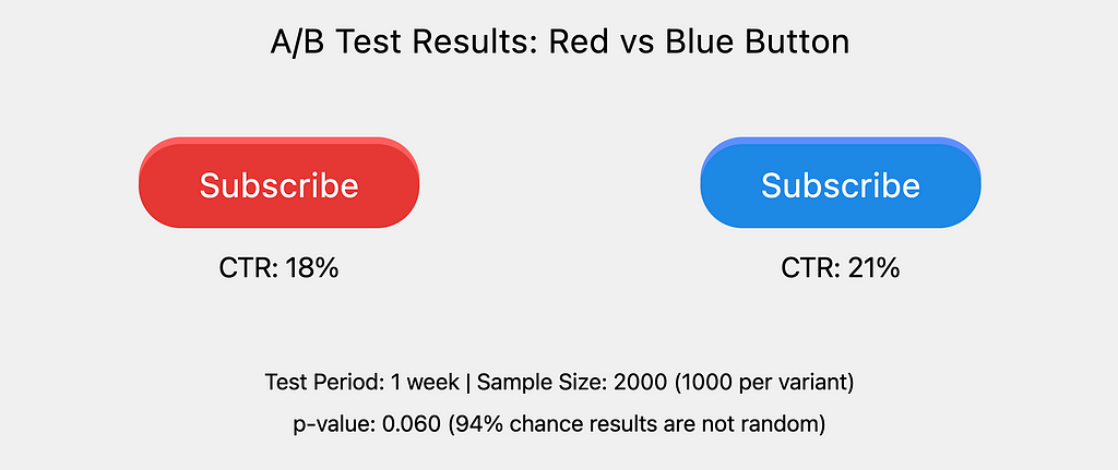
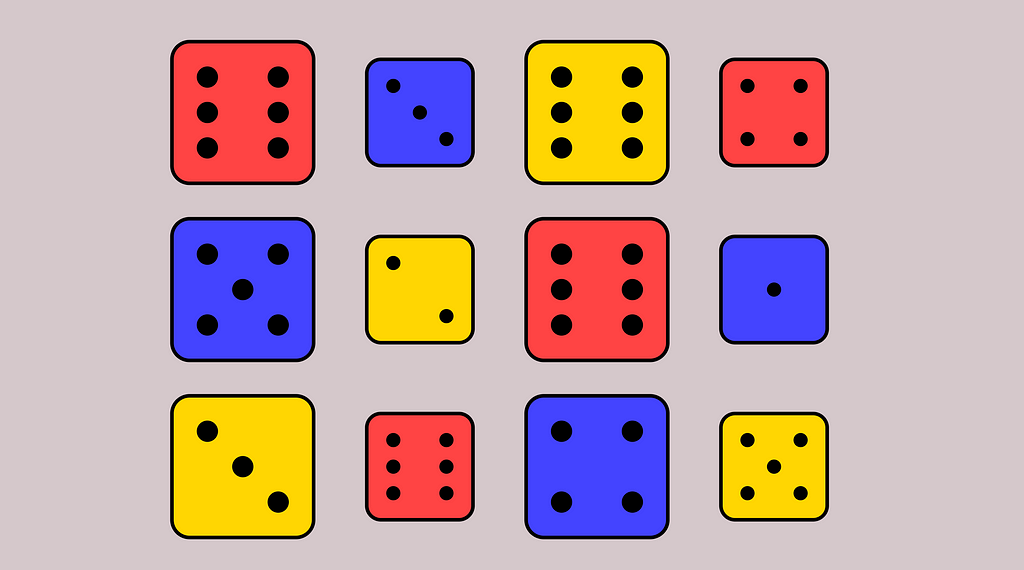
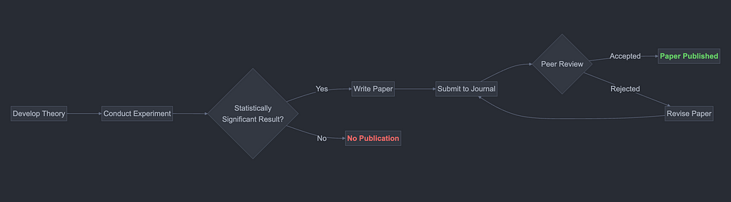


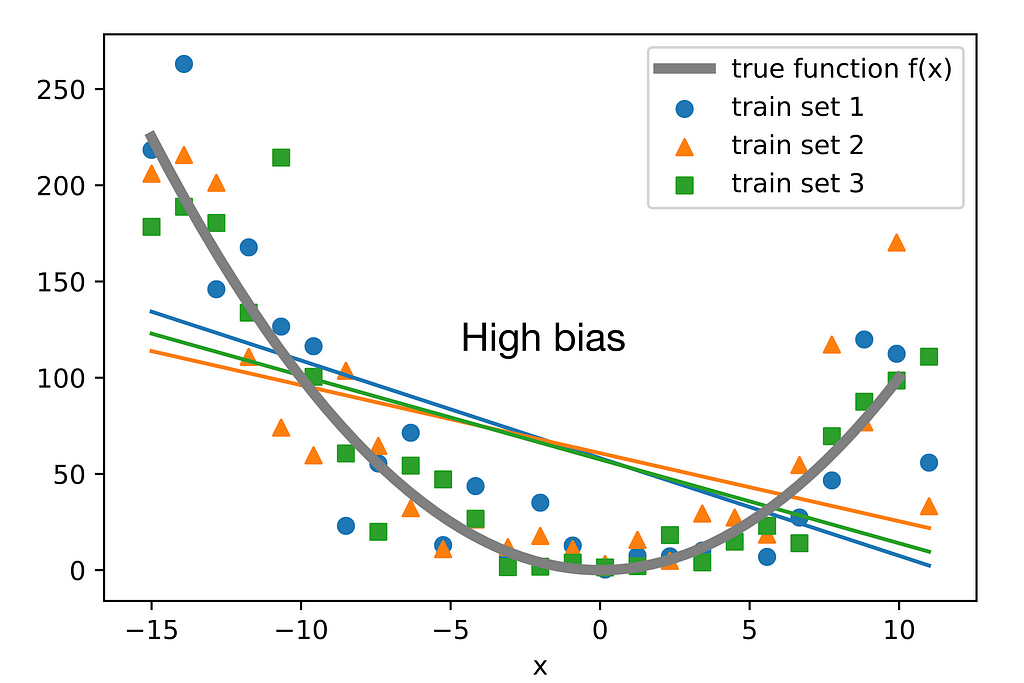
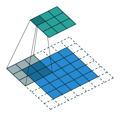
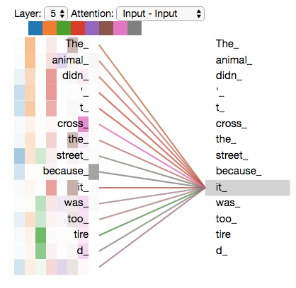


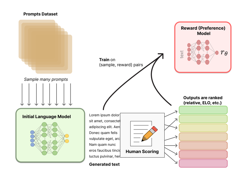


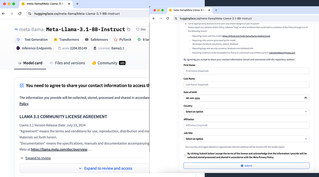
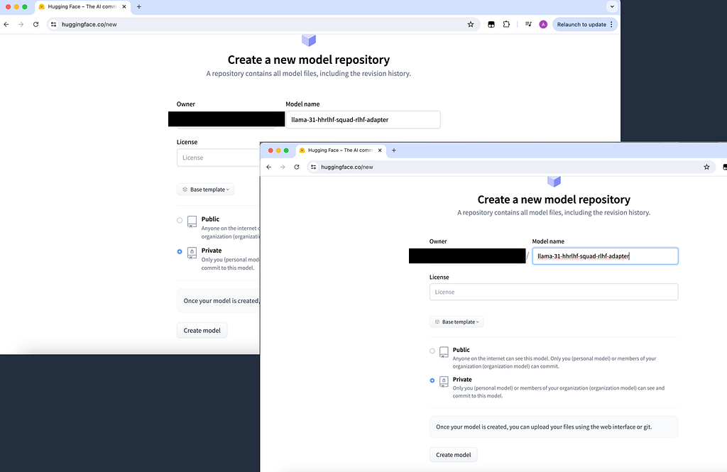
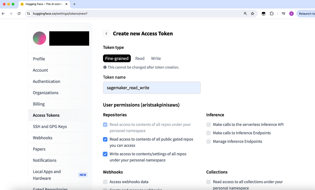


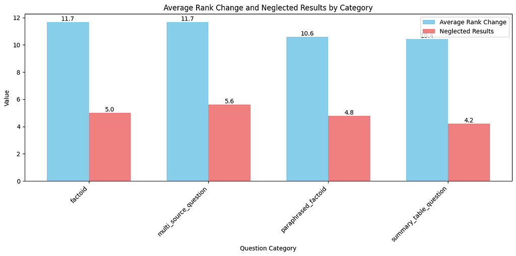
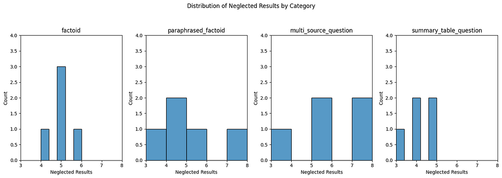
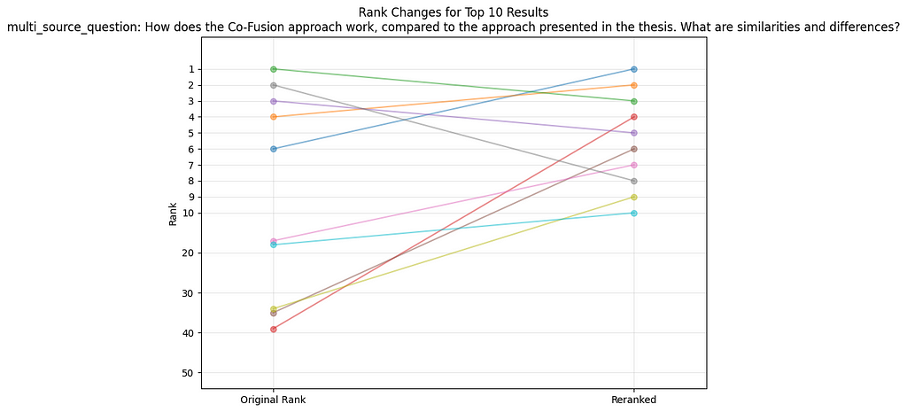
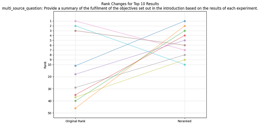


