Two short anecdotes about transformations, and what it takes if you want to become ”AI-enabled”
Generated by ChatGTP
Many product companies I talk to struggle to understand what “transformation to AI” means to them. In this post, I share some insights into what it means to be an AI-enabled business, and what you can do to get there. Not by enumerating things you have to do, but through two anecdotes. The first is about digitalisation — what it means for a non-digital company to transform into a digital company. This is because the transition to AI follows the same kind of path; it is a “same same but different” transformation. The second story is about why so many product companies failed in their investments in AI and Data Science over the last years, because they put AI in a corner.
But before we go there, keep in mind that becoming AI-enabled is a transformation, or a journey. And to embark upon a journey and successfully riding along to its destination, you are better off knowing where you are going. So: what what does it mean to be “AI-enabled”?
To be AI-enabled is to be able to use AI technology to seize an opportunity, or to obtain a competitive advantage, that you could otherwise not.
So, after finishing the transformation, how can you know whether you have succeeded? You ask yourself the question:
What can we do now that we could not do before? Can we take advantage of an opportunity now, that we could not before?
Or more to the point: *Will* we take advantage of an opportunity now, that we could not before?
There is nothing AI-specific about this question. It is valid for any transformation an organisation takes upon itself in order to acquire new capabilities. And, for this very reason, there is a lot to learn from other transformations, if you wish to transition to AI.
Anecdote 1: A tale of digitalisation
Generated by ChatGPT
Over the last decades, there has been a tremendous shift in some large businesses referred to as digitalisation. This is the process where a company transforms from using IT as a tool in their everyday work, to using IT as a strategic asset to achieve competitive advantage. A few years back, I spent some time in the Oil & Gas sector, participating in large digitalisation efforts. And if you have not worked in O&G, you may be surprised to learn that this huge economy still is not digital, to a large extent. Of course, the sector has used computers since they came about, but as tools: CAD-tools for design, logistics systems for project and production planning, CRM systems for managing employees and customers, and so on. But the competitive power of one company over another has been in their employees’ knowledge about steel and pipes and machinery, about how fluids flows through pipes, about installation of heavy equipment under rough conditions, and many other things of this trade. Computers have been perceived as tools to get the job done, and IT has been considered an expense to be minimised. Digitalisation is the transformation that aims to change that mindset.
To enable IT as leverage in competition, the business must move from thinking about IT as an expense, to thinking of IT as an investment opportunity. By investing in your own IT, you can create tools and products that competitors do not have, and that give you a competitive advantage.
But investing in in-house software development is expensive, so to pin down the right investments to shift competition in your favour, you need all the engineers, the steel and machinery specialists, to start thinking about which problems and challenges you can solve with computers in a manner that serves this cause. This is because, the knowledge about how to improve your products and services, is located in the heads of the employees: the sales people talking to the customers, the marketing people feeling the market trends on their fingertips, the product people designing and manufacturing the assets, and the engineers designing, making and testing the final product artefacts. These humans must internalise the idea of using computer technology to improve the business as a whole, and do it. That is the goal of digitalisation.
But you already knew this, right? So why bother reiterating?
Because a transformation to AI is the exact same story over again; you just have to replace “digital transformation” by “transformation to AI”. Hence, there is much to learn from digitalisation programs. And if you are lucky, you already understand what it means to be a digital company, so you actually know what a transformation to digital entails.
Anecdote 2: The three eras of Data Science
Generated by ChatGPT
The history of industrial AI and Data Science is short, starting back in 2010–2012. While there is some learning to be had from this history, I’ll say right away: there is still no silver bullet for going AI with a bang. But, as an industry, we are getting better at it. I think of this history as playing out over three distinct eras, demarcated by how many companies approached AI when they launched their first AI initiatives.
In the first era, companies that wanted to use AI and ML invested heavily in large data infrastructures and hired a bunch of data scientists, placed them in a room, and waited for magic to emanate. But nothing happened, and the infrastructure and the people were really expensive, so the method was soon abandoned. The angle of attack was inspired by large successes such as Twitter, Facebook, Netflix, and Google, but the scale of these operations don’t apply to most companies. Lesson learned.
In the second era, having learned from the first era, the AI advisors said that you should start by identifying the killer AI-app in your domain, hire a small team of Data Scientists, make an MVP, and iterate from there. This would give you a high-value project and star example with which you could demonstrate the magnificence of AI to the entire company. Everybody would be flabbergasted, see the light, and the AI transformation would be complete. So companies hired a small team of data scientists, placed them in a corner, and waited for magic to emanate. But nothing happened.
And the reason why magic does not happen in this setting is that the data scientists and AI/ML experts hired to help in the transformation don’t know the business. They know neither your nor your customer’s pain points. They don’t know the hopes, dreams, and ambitions of the business segment. And, moreover, the people who know this, the product people, managers, and engineers in your organisation, they don’t know the data scientists, or AI, or what AI can be used for. And they don’t understand what the Data Scientists are saying. And before these groups learn to talk with each other, there will be no magic. Because, before that, no AI transformation has taken place.
This is why it is important to ask, not what you can do, but what you will do, when you check whether you have transformed or not. The AI team can help in applying AI to seize an opportunity, but it will not happen unless they know what to do.
This is a matter of communication. Of getting the right people to talk to each other. But communication across these kinds of boundaries is challenging, leading us to where we are now:
The third era — While still short of a silver bullet, the current advice goes as follows:
Get hold of someone experienced with AI and machine learning. It is a specialist discipline, and you need the competency. Unless you are sitting on exceptional talent, don’t try to turn your other-area experts into Data Scientists over night. Building a team from scratch takes time, and they will have no experience at the onset. Don’t hesitate to go externally to find someone to help you get started.
Put the Data Scientists in touch with your domain experts and product development teams, and let them, together, come up with the first AI application in your business. It does not have to be the killer app — if you can find anything that may be of use, it will do.
Go ahead and develop the solution and showcase it to the rest of the organisation.
The point of the exercise is not to strike bullseye, but to set forth a working AI example that the rest of the organisation can recognise, understand, and critique. If the domain experts and the product people come forth saying “But you solved the wrong problem! What you should have done is…” you can consider it a victory. By then, you have the key resources talking to each other, collaborating to find new and better solutions to the problems you already have set out to solve.
During my time as a Data Scientist, the “Data Scientist in the corner” pitfall is one of the main reasons groups or organisations fail in their initial AI-initiatives. Not having the AI-resources interacting closely with the product teams should be considered rigging for failure. You need the AI-initiatives to be driven by the product teams — that is how you ensure that the AI solutions contribute to solving the right problems.
Summing up
The transformation to being an AI-enabled product organisation builds on top of being digitally enabled, and follows the same kind of path: The key to success is in engaging with the domain experts and the product teams, getting them up and running on the extended problem solving capabilities provided by AI.
AI and Machine Learning is a complicated specialist discipline, and you need someone proficient in the craft. Thereafter, the key is to deeply connect that resource with the domain experts and product teams, so that they can start solving problems together.
And: don’t put AI in a corner!
The process of transformation. Illustration by the author in collaboration with ChatGPT and GIMP.
Aligning expectations with reality by using traditional ML to bridge the gap in a LLM’s responses
Early on we all realized that LLMs only knew what was in their training data. Playing around with them was fun, sure, but they were and still are prone to hallucinations. Using such a product in its “raw” form commercially is to put it nicely — dumb as rocks (the LLM, not you… possibly). To try alleviate both the issues of hallucinations and having knowledge of unseen/private data, two main avenues can be taken. Train a custom LLM on your private data (aka the hard way), or use retrieval augmentation generation (aka the one we all basically took).
RAG is an acronym now widely used in the field of NLP and generative AI. It has evolved and led to many diverse new forms and approaches such as GraphRAG, pivoting away from the naive approach most of us first started with. The me from two years ago would just parse raw documents into a simple RAG, and then on retrieval, provide this possible (most likely) junk context to the LLM, hoping that it would be able to make sense of it, and use it to better answer the user’s question. Wow, how ignorance is bliss; also, don’t judge: we all did this. We all soon realized that “garbage in, garbage out” as our first proof-of-concepts performed… well… not so great. From this, much effort was put in by the open-source community to provide us ways to make a more sensible commercially viable application. These included, for example: reranking, semantic routing, guardrails, better document parsing, realigning the user’s question to retrieve more relevant documents, context compression, and the list could go on and on. Also, on top of this, we all 1-upped our classical NLP skills and drafted guidelines for teams curating knowledge so that the parsed documents stored in our databases were now all pretty and legible.
While working on a retrieval system that had about 16 (possible exaggeration) steps, one question kept coming up. Can my stored context really answer this question? Or to put it another way, and the one I prefer. Does this question really belong to the stored context? While the two questions seem similar, the distinction lies with the first being localized (e.g. the 10 retrieved docs) and the other globalized (with respect to the entire subject/topic space of the document database). You can think of them as one being a fine-grained filter while the other is more general. I’m sure you’re probably wondering now, but what is the point of all this? “I do cosine similarity thresholding on my retrieved docs, and everything works fine. Why are you trying to complicate things here?” OK, I made up that last thought-sentence, I know that you aren’t that mean.
To drive home my over-complication, here is an example. Say that the user asks, “Who was the first man on the moon?” Now, let’s forget that the LLM could straight up answer this one and we expect our RAG to provide context for the question… except, all our docs are about products for a fashion brand! Silly example, agreed, but in production many of us have seen that users tend to ask questions all the time that don’t align with any of the docs we have. “Yeah, but my pretext tells the LLM to ignore questions that don’t fall within a topic category. And the cosine similarity will filter out weak context for these kinds of questions anyways” or “I have catered for this using guardrails or semantic routing.” Sure, again, agreed. All these methods work, but all these options either do this too late downstream e.g. the first two examples or aren’t completely tailored for this e.g. the last two examples. What we really need is a fast classification method that can rapidly tell you if the question is “yea” or “nay” for the docs to provide context for… even before retrieving them. If you’ve guessed where this is going, you’re part of the classical ML crew 😉 Yep, that’s right, good ole outlier detection!
Outlier detection combined with NLP? Clearly someone has wayyyy too much free time to play around.
When building a production level RAG system, there are a few things that we want to make sure: efficiency (how long does a response usually take), accuracy (is the response correct and relevant), and repeatability (sometimes overlooked, but super important, check a caching library for this one). So how is an outlier detection method (OD) going to help with any of these? Let’s brainstorm quick. If the OD sees a question and immediately says “nay, it’s on outlier” (I’m anthropomorphizing here) then many steps can be skipped later downstream making this route way more efficient. Say now that the OD says “yea, all safe”, well, with a little overhead we can have a greater level of assurance that the topic space of both the question and the stored docs are aligned. With respect to repeatability, well we’re in luck again, since classic ML methods are generally repeatable so at least this additional step isn’t going to suddenly start apologizing and take us on a downward spiral of repetition and misunderstanding (I’m looking at you ChatGPT).
Wow, this has been a little long-winded, sorry, but finally I can now start showing you the cool stuff.
Muzlin, a python library, a project which I am actively involved in, has been developed exactly for these type of semantic filtering tasks by using simple ML for production ready environments. Skeptical? Well come on, let’s take a quick tour of what it can do for us.
The dataset that we will be working with is a dataset of 5.18K rows from BEIR (Scifact, CC BY-SA 4.0). To create a vectorstore we will use the scientific claim column.
So, with the data loaded (a bit of a small one, but hey this is just a demo!) the next step is to encode it. There are many ways in which to do this e.g. tokenizing, vector embeddings, graph node-entity relations, and more, but for this simple example let’s use vector embeddings. Muzlin has built-in support for all the popular brands (Apple, Microsoft, Google, OpenAI), well I mean their associated embedding models, but you get me. Let’s go with, hmmm, HuggingFace, because you know, it’s free and my current POC budget is… as shoestring as it gets.
Sweet! If you can believe it, we’re already halfway there. Is it just me, or do so many of these LLM libraries leave you having to code an extra 1000 lines with a million dependencies only to break whenever your boss wants a demo? It’s not just me, right? Right? Anyways, rant aside there are really just two more steps to having our filter up and running. The first, is to use an outlier detection method to evaluate the embedded vectors. This allows for an unsupervised model to be constructed that will give you a likelihood value of how possible any given vector in our current or new embeddings are.
No jokes, that’s it. Your model is all done. Muzlin is fully Sklearn compatible and Pydantically validated. What’s more, MLFlow is also fully integrated for data-logging. The example above is not using it, so this result will automatically generate a joblib model in your local directory instead. Niffy, right? Currently only PyOD models are supported for this type of OD, but who knows what the future has in store.
Damn Daniel, why you making this so easy. Bet you’ve been leading me on and it’s all downhill from here.
In response to above, s..u..r..e that meme is getting way too old now. But otherwise, no jokes, the last step is at hand and it’s about as easy as all the others.
Okay, okay, this was the longest script, but look… most of it is just to play around with it. But let’s break down what’s happening here. First, the OutlierDetector class is now expecting a model. I swear it’s not a bug, it’s a feature! In production you don’t exactly want to train the model each time on the spot just to inference, and often the training and inferencing take place on different compute instances, especially on cloud compute. So, the OutlierDetector class caters for this by letting you load an already trained model so you can inference on the go. YOLO. All you have to do now is just encode a user’s question and predict using the OD model, and hey presto well looky here, we gots ourselves a little outlier.
What does this mean now that the user’s question is an outlier? Cool thing, that’s all up to you to decide. The stored documents most likely do not have any context to provide that would answer said question in any meaningful way. And you can rather reroute this to either tell that Kyle from the testing team to stop messing around, or more seriously save tokens and have a default response like “I’m sorry Dave, I’m afraid I can’t do that” (oh HAL 9000 you’re so funny, also please don’t space me).
To sum everything up, integration is better (Ha, math joke for you math readers). But really, classical ML has been around way longer and is way more trustworthy in a production setting. I believe more tools should incorporate this ethos going forward on the generative AI roller-coaster ride we’re all on, (side note, this ride costs way too many tokens). By using outlier detection, off-topic queries can quickly be rerouted saving compute and generative costs. As an added bonus I’ve even provided an option to do this with GraphRAGs too, heck yeah — nerds unite! Go forth, and enjoy the tools that open source devs lose way too much sleep to give away freely. Bon voyage and remember to have fun!
This article aims to explain the fundamentals of parallel computing. We start with the basics, including understanding shared vs. distributed architectures and communication within these systems. We will explore GPU architecture and how coding elements (using C++ Kokkos) help map architectural principles to code implementation. Finally, we will measure performance metrics (speedup) using the runtime data obtained from running the Kokkos code on both CPU and GPU architectures for vector-matrix multiplication, one of the most common operations in the machine learning domain.
The central theme of the article is exploring and answering questions. It may seem like a lengthy journey, but it will be worth it. Let’s get started!
Fundamentals of System Architecture
I get that parallel computing saves time by running multiple operations at once. But I’ve heard that system time is different from human time or wall-clock time. How is it different?
The smallest unit of time in computing is called a clock tick. It represents the minimum time required to perform an operation, such as fetching data, executing computations, or during communication. A clock tick technically refers to the change of state necessary for an instruction.The state can be processor state, data state, memory state, or control signals.In one clock tick, a complete instruction, part of an instruction, or multiple instructions may be executed.
CPU allows for a limited number of state changes per second. For example, a CPU with 3GHz clock speed allows for 3 billion changes of state per second. There is a limit to the allowable clock speed because each clock tick generates heat, and excessive speed can damage the CPU chip due to the heat generated.
Therefore, we want to utilize the available capacity by using parallel computing methodologies. The purpose is to hide memory latency (the time it takes for the first data to arrive from memory), increase memory bandwidth (the amount of data transferred per unit of time), and enhance compute throughput (the tasks performed in a clock tick).
To compare performance, such as when calculating efficiency of a parallel program, we use wall-clock time instead of clock ticks, since it includes all real-time overheads like memory latency and communication delays, that cannot be directly translated to clock ticks.
What does the architecture of a basic system look like?
A system can consist of a single processor, a node, or even a cluster. Some of the physical building blocks of a system are —
Node — A physical computer unit that has several processor chips. Multiple nodes combine to form a cluster.
Processor Chips — Chips contain multiple processing elements called cores.
Core — Each core is capable of running an independent thread of execution.
In set terms, a node can have a one-to-many relationship with processor chips, and each processor chip can have a one-to-many relationship with cores. The image below gives a visual description of a node with processors and cores.
Modern node with four eight-core processors that share a common memory pool. Ref: Cornell Virtual Workshop
The non-physical components of a system include threads and processes —
Thread — Thread is a sequence of CPU instructions that operating system treats as a single unit for scheduling and execution purposes.
Process — In computing, a process is a coherent unit of resource allocation, including memory, file handlers, ports and devices. A single process may manage resources for several threads. Threads can be modelled as components of a process.
So, do threads run on cores on the same system, or can they be spread across different systems for a single program? And in either case, how do they communicate? How’s memory handled for these threads ? Do they share it, or do they each get their own separate memory?
A single program can execute across multiple cores on the same or different systems/ nodes. The design of the system and the program determines whether it aligns with the desired execution strategy.
When designing a system, three key aspects must be considered: execution (how threads run), memory access (how memory is allocated to these threads), and communication (how threads communicate, especially when they need to update the same data). It’s important to note that these aspects are mostly interdependent.
Execution
Serial execution— This uses a single thread of execution to work on a single data item at any time.
Parallel execution — In this, more than one thing happens simultaneously. In computing, this can be —
One worker — A single thread of execution operating on multiple data items simultaneously (vector instructions in a CPU). Imagine a single person sorting a deck of cards by suit. With four suits to categorize, the individual must go through the entire deck to organize the cards for each suit.
Working Together — Multiple threads of execution in a single process. It is equivalent to multiple people working together to sort a single deck of cards by suit.
Working Independently — Multiple processes can work on the same problem, utilizing either the same node or multiple nodes. In this scenario, each person would be sorting their deck of cards.
Any combination of the above.
Working Together: Two workers need to insert cards from the same suit. Worker A is holding the partial results for the clubs suit, so Worker B is temporarily blocked. Ref: Cornell Virtual Workshop
Memory Access
Shared Memory — When a program runs on multiple cores (a single multithreaded process) on the same system, each thread within the process has access to memory in the same virtual address space.
Distributed Memory — A distributed memory design is employed when a program utilizes multiple processes (whether on a single node or across different nodes). In this architecture, each process owns a portion of the data, and other processes must send messages to the owner to update their respective parts. Even when multiple processes run on a single node, each has its own virtual memory space. Therefore, such processes should use distributed memory programming for communication.
Hybrid Strategy — Multithreaded processes that can run on the same or different nodes, designed to use multiple cores on a single node through shared memory programming. At the same time, they can employ distributed memory strategies to coordinate with processes on other nodes. Imagine multiple people or threads working in multiple cubicles in the image above. Workers in the same cubicle communicate using shared memory programming, while those in different cubicles interact through distributed memory programming.
In a distributed memory design, parallel workers are assigned to different cubicles (processes). Ref: Cornell Virtual Workshop
Communication
The communication mechanism depends on the memory architecture. In shared memory architectures, application programming interfaces like OpenMP (Open Multi-Processing)enable communication between threads that share memory and data. On the other hand, MPI (Message Passing Interface) can be used for communication between processes running on the same or different nodes in distributed memory architectures.
Parallelization Strategy and Performance
How can we tell if our parallelization strategy is working effectively?
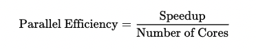
There are several methods, but here, we discuss efficiency and speedup. In parallel computing, efficiency refers to the proportion of available resources that are actively utilized during a computation. It is determined by comparing the actual resource utilization against the peak performance, i.e., optimal resource utilization.
Actual processor utilization refers to the number of floating point operations (FLOP) performed over a specific period.
Peak performance assumes that each processor core executes the maximum possible FLOPs during every clock cycle.
Efficiency for parallel code is the ratio of actual floating-point operations per second (FLOPS) to the peak possible performance.
Speedup is used to assess efficiency and is measured as:
Suppose the serial execution of code took 300 seconds. After parallelizing the tasks using 50 cores, the overall wall-clocktime for parallel execution was 6 seconds. In this case, the speedup can be calculated as the wall-clock time for serial execution divided by the wall-clock time for parallel execution, resulting in a speedup of 300s/6s = 50. We get parallel efficiency by dividing the speedup by the number of cores, 50/50 = 1. This is an example of the best-case scenario: the workload is perfectly parallelized, and all cores are utilized efficiently.
Will adding more computing units constantly improve performance if the data size or number of tasks increases?
Only sometimes. In parallel computing, we have two types of scaling based on the problem size or the number of parallel tasks.
Strong Scaling — Increasing the number of parallel tasks while keeping the problem size constant. However, even as we increase the number of computational units (cores, processors, or nodes) to process more tasks in parallel, there is an overhead associated with communication between these units or the host program, such as the time spent sending and receiving data.
Ideally, the execution time decreases as the number of parallel tasks increases. However, if the code doesn’t get faster with strong scaling, it could indicate that we’re using too many tasks for the amount of work being done.
Weak Scaling — In this, problem size increases as the number of tasks increase, so computation per task remains constant. If your program has good weak scaling performance, you can run a problem twice as large on twice as many nodes in the same wall-clock time.
There are restrictions around what we can parallelize since some operations can’t be parallelized. Is that right?
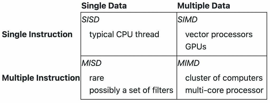
Yes, parallelizing certain sequential operations can be quite challenging. Parallelizing depends on multiple instruction streams and/or multiple data streams.
To understand what can be parallelized, let’s look at SIMD in CPUs, which is achieved using vectorization.
Vectorization is a programming technique in which operations are applied to entire arrays at once rather than processing individual elements one by one. It is achieved using the vector unit in processors, which includes vector registers and vector instructions.
Consider a scenario where we iterate over an array and perform multiple operations on a single element within a for loop. When the data is independent, writing vectorizable code becomes straightforward; see the example below:
do i, n
  a(i) = b(i) + c(i)
  d(i) = e(i) + f(i)
end do
In this loop, each iteration is independent — meaning a(i) is processed independently of a(i+1) and so on. Therefore, this code is vectorizable, that will allow multiple elements of array a to be computed in parallel using elements from b and c, as demonstrated below:
Data dependencies commonly encountered in scientific code are –
Read After Write (RAW) — Not Vectorizable
do i, n
  a(i) = a(i-1) +b(i)
Write After Read (WAR) — Vectorizable
do i, n
  a(i) = a(i+1) +b(i)
Write After Write (WAW) — Not Vectorizable
do i, n
  a(i%2) = a(i+1) +b(i)
Read After Read (RAR) — Vectorizable
do i, n
  a(i) = b(i%2) + c(i)
Adhering to certain standard rules for vectorization — such as ensuring independent assignments in loop iterations, avoiding random data access, and preventing dependencies between iterations — can help write vectorizable code.
GPU architecture and cross-architectural code
When data increases, it makes sense to parallelize as many parallelizable operations as possible to create scalable solutions, but that means we need bigger systems with lots of cores. Is that why we use GPUs? How are they different from CPUs, and what leads to their high throughput?
YES!
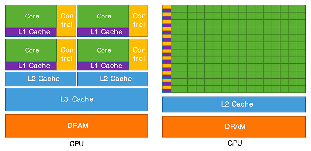
Comparing the relative capabilities of the basic elements of CPU and GPU architectures. Ref: Cornell Virtual Workshop
GPUs (Graphics processing units) have many more processor units (green) and higher aggregate memory bandwidth (the amount of data transferred per unit of time) as compared to CPUs, which, on the other hand, have more sophisticated instruction processing and faster clock speed. As seen above, CPUs have more cache memory than GPUs. However, CPUs have fewer arithmetic logic units (ALUs) and floating point units (FPUs) than GPUs. Considering these points, using CPUs for complex workflow and GPUs for computationally intensive tasks is intuitive.
GPUs are designed to produce high computational throughput using their massively parallel architecture. Their computational potential can be measured in billions of floating point operations per second (GFLOPS). GPU hardware comes in the form of standard graphic cards (NVIDIA quad), High-end accelerator cards (NVIDIA Tesla), etc.
Two key properties of the graphics pipeline that enable parallelization and, thus, high throughput are —
Independence of Objects — A typical graphics scene consists of many independent objects; each object can be processed separately without dependencies on the others.
Uniform Processing Steps — The sequence of processing steps is the same for all objects.
So, multiple cores of GPUs work on different data at the same time, executing computations in parallel like a SIMD (Single Instruction Multiple Data) architecture. How are tasks divided between cores? Does each core run a single thread like in the CPU?
In a GPU, Streaming Multiprocessors (SMs) are similar to cores in a CPU. Cores in GPUs are similar to vector lanes in CPUs. SMs are the hardware units that house cores.
When a function or computation, referred as a kernel, is executed on the GPU, it is often broken down into thread blocks. These thread blocks contain multiple threads; each SM can manage many threads across its cores. If there are more thread blocks than SMs, multiple thread blocks can be assigned to a single SM. Also, multiple threads can run on a single core.
Each SM further divides the thread blocks into groups called warps, with each warp consisting of 32 threads. These threads execute the same stream of instructions on different data elements, following a Single Instruction, Multiple Data (SIMD) model. The warp size is set to 32 because, in NVIDIA’s architecture, CUDA cores are grouped into sets of 32. This enables all threads in a warp to be processed together in parallel by the 32 CUDA cores, achieving high efficiency and optimized resource utilization.
In SIMD (Single Instruction, Multiple Data), a single instruction acts uniformly on all data elements, with each data element processed in exactly the same way. SIMT (Single Instruction, Multiple Threads), which is commonly used in GPUs, relaxes this restriction. In SIMT, threads can be activated or deactivated so that instruction and data are processed in active threads; however, the local data remains unchanged on inactive threads.
I want to understand how we can code to use different architectures. Can similar code work for both CPU and GPU architectures? What parameters and methods can we use to ensure that the code efficiently utilizes the underlying hardware architecture, whether it’s CPUs or GPUs?
Code is generally written in high-level languages like C or C++ and must be converted into binary code by a compiler since machines cannot directly process high-level instructions. While both GPUs and CPUs can execute the same kernel, as we will see in the example code, we need to use directives or parameters to run the code on a specific architecture to compile and generate an instruction set for that architecture. This approach allows us to use architecture-specific capabilities. To ensure compatibility, we can specify the appropriate flags for the compiler to produce binary code optimized for the desired architecture, whether it is a CPU or a GPU.
Various coding frameworks, such as SYCL, CUDA, and Kokkos, are used to write kernels or functions for different architectures. In this article, we will use examples from Kokkos.
A bit about Kokkos — An open-source C++ programming model for performance portability for writing Kernels: it is implemented as a template library on top of CUDA, OpenMP, and other backends and aims to be descriptive, in the sense that we define what we want to do rather than prescriptive (how we want to do it). Kokkos Core provides a programming model for parallel algorithms that uses many-core chips and shares memory across those cores.
A kernel has three components —
Pattern — Structure of the computation: for, scan, reduction, task-graph
Execution policy — How computations are executed: static scheduling, dynamic scheduling, thread teams.
Computational Body — Code which performs each unit of work. e.g., loop body
Pattern and policy drive computational body. In the example below, used just for illustration, ‘for’ is the pattern, the condition to control the pattern (element=0; element<n; ++element) is the policy, and the computational body is the code executed within the pattern
for (element=0; element<n; ++element){
  total = 0;
  for(qp = 0; qp < numQPs; ++qp){
    total += dot(left[element][qp], right[element][qp]);
  }
  elementValues[element] = total;
}
The Kokkos framework allows developers to define parameters and methods based on three key factors: where the code will run (Execution Space), what memory resources will be utilized (Memory Space), and how data will be structured and managed (Data Structure and Data management).
We primarily discuss how to write the Kokkos kernel for the vector-matrix product to understand how these factors are implemented for different architectures.
But before that, let’s discuss the building blocks of the kernel we want to write.
Memory Space —
Kokkos provides a range of memory space options that enable users to control memory management and data placement on different computing platforms. Some commonly used memory spaces are —
HostSpace — This memory space represents the CPU’s main memory. It is used for computations on the CPU and is typically the default memory space when working on a CPU-based system.
CudaSpace — CudaSpace is used for NVIDIA GPUs with CUDA. It provides memory allocation and management for GPU devices, allowing for efficient data transfer and computation.
CudaUVMSpac — For Unified Virtual Memory (UVM) systems, such as those on some NVIDIA GPUs, CudaUVMSpace enables the allocation of memory accessible from both the CPU and GPU without explicit data transfers. Cuda runtime automatically handles data movement at a performance hit.
It is also essential to discuss memory layout, which refers to the organization and arrangement of data in memory. Kokkos provides several memory layout options to help users optimize their data storage for various computations. Some commonly used memory layouts are —
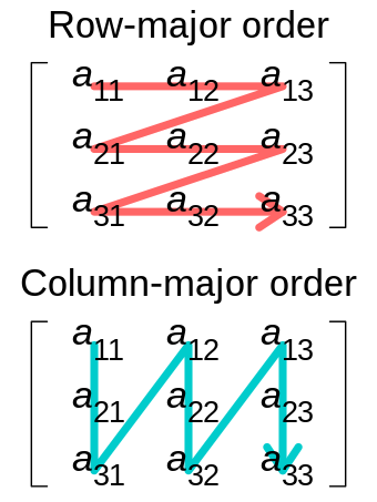
Row-major vs Column-major iteration of a matrix. Ref: Wikipedia
LayoutRight (also known as Row-Major) is the default memory layout for multi-dimensional arrays in C and C++. In LayoutRight, the rightmost index varies most rapidly in memory. If no layout is chosen, the default layout for HostSpace is LayoutRight.
LayoutLeft (also known as Column-Major) — In LayoutLeft, the leftmost index varies most rapidly in memory. If no layout is chosen, the default layout for CudaSpace is LayoutLeft.
In the programmatic implementation below, we defined memory space and layout as macros based on the compiler flag ENABLE_CUDA, which will be True if we want to run our code on GPU and False for CPU.
    // ENABLE_CUDA is a compile time argument with default value true
    #define ENABLE_CUDA true

    // If CUDA is enabled, run the kernel on the CUDA (GPU) architecture
    #if defined(ENABLE_CUDA) && ENABLE_CUDA
        #define MemSpace Kokkos::CudaSpace
        #define Layout Kokkos::LayoutLeft
    #else
    // Define default values or behavior when ENABLE_CUDA is not set or is false
        #define MemSpace Kokkos::HostSpace
        #define Layout Kokkos::LayoutRight
    #endif
Data Structure and Data Management —
Kokkos Views — In Kokkos, a “view” is a fundamental data structure representing one-dimensional and multi-dimensional arrays, which can be used to store and access data efficiently. Kokkos views provide a high-level abstraction for managing data and is designed to work seamlessly with different execution spaces and memory layouts.
    // View for a 2d array of data type double
    Kokkos::View<double**> myView("myView", numRows, numCols);
    // Access Views
    myView(i, j) = 42.0;
    double value = myView(i, j);
Kokkos Mirroring technique for data management — Mirrors are views of equivalent arrays residing in possible different memory spaces, which is when we need data in both CPU and GPU architecture. This technique is helpful for scenarios like reading data from a file on the CPU and subsequently processing it on the GPU. Kokkos’ mirroring creates a mirrored view of the data, allowing seamless sharing between the CPU and GPU execution spaces and facilitating data transfer and synchronization.
To create a mirrored copy of the primary data, we can use Kokkos’ create_mirror_view() function. This function generates a mirror view in a specified execution space (e.g., GPU) with the same data type and dimensions as the primary view.
    // Intended Computation -
    // <y, A*x> = y^T * A * x
    // Here:
    // y and x are vectors.
    // A is a matrix.

    // Allocate y, x vectors and Matrix A on device
    typedef Kokkos::View<double*, Layout, MemSpace>   ViewVectorType;
    typedef Kokkos::View<double**, Layout, MemSpace>  ViewMatrixType;

    // N and M are number of rows and columns
    ViewVectorType y( "y", N );
    ViewVectorType x( "x", M );
    ViewMatrixType A( "A", N, M );

    // Create host mirrors of device views
    ViewVectorType::HostMirror h_y = Kokkos::create_mirror_view( y );
    ViewVectorType::HostMirror h_x = Kokkos::create_mirror_view( x );
    ViewMatrixType::HostMirror h_A = Kokkos::create_mirror_view( A );

    // Initialize y vector on host.
    for ( int i = 0; i < N; ++i ) {
        h_y( i ) = 1;
    }

    // Initialize x vector on host.
    for ( int i = 0; i < M; ++i ) {
        h_x( i ) = 1;
    }

    // Initialize A matrix on host.
    for ( int j = 0; j < N; ++j ) {
        for ( int i = 0; i < M; ++i ) {
            h_A( j, i ) = 1;
        }
    }

    // Deep copy host views to device views.
    Kokkos::deep_copy( y, h_y );
    Kokkos::deep_copy( x, h_x );
    Kokkos::deep_copy( A, h_A );
Execution Space —
In Kokkos, the execution space refers to the specific computing environment or hardware platform where parallel operations and computations are executed. Kokkos abstracts the execution space, enabling code to be written in a descriptive manner while adapting to various hardware platforms.
We discuss two primary execution spaces —
Serial: The Serial execution space is a primary and portable option suitable for single-threaded CPU execution. It is often used for debugging, testing, and as a baseline for performance comparisons.
Cuda: The Cuda execution space is used for NVIDIA GPUs and relies on CUDA technology for parallel processing. It enables efficient GPU acceleration and management of GPU memory.
Either the ExecSpace can be defined, or it can be determined dynamically based on the Memory space as below:
// Execution space determined based on MemorySpace
using ExecSpace = MemSpace::execution_space;
How can we use these building blocks to write an actual kernel? Can we use it to compare performance between different architectures?
For the purpose of writing a kernel and performance comparison, we use following computation:
<y, A*x> = y^T * (A * x)

Here:

y and x are vectors.

A is a matrix.

<y, A*x> represents the inner product or dot product of vectors y
and the result of the matrix-vector multiplication A*x.

y^T denotes the transpose of vector y.

* denotes matrix-vector multiplication.
The kernel for this operation in Kokkos —
    // Use a RangePolicy.
    typedef Kokkos::RangePolicy<ExecSpace>  range_policy;

    // The below code is run for multiple iterations across different
    // architectures for time comparison
    Kokkos::parallel_reduce( "yAx", range_policy( 0, N ),
                KOKKOS_LAMBDA ( int j, double &update ) {
                    double temp2 = 0;

                    for ( int i = 0; i < M; ++i ) {
                        temp2 += A( j, i ) * x( i );
                    }
                    update += y( j ) * temp2;
            }, result );
For the above kernel, parallel_reduce serves as the pattern, range_policy defines the policy, and the actual operations constitute the computational body.
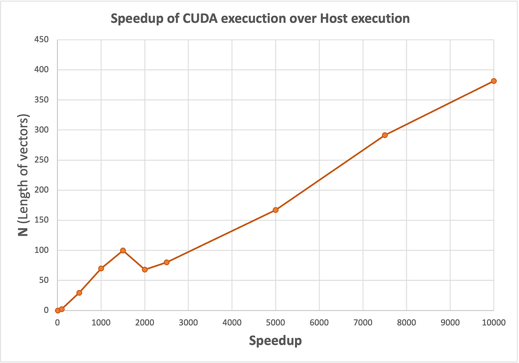
I executed this kernel on a TACC Frontera node which has an NVIDIA Quadro RTX 5000 GPU. The experiments were performed with varying values of N, which refers to the lengths of the vectors y and x, and the number of rows in matrix A. Computation was performed 100 times to get notable results, and the execution time of the kernel was recorded for both Serial (Host) and CUDA execution spaces. I used ENABLE_CUDA compiler flag to switch between execution environments: True for GPU/CUDA execution space and False for CPU/serial execution space. The results of these experiments are presented below, with the corresponding speedup.
Speedup trend for varying data size (GPU vs CPU) Ref: Image by author
We notice that the speedup increases significantly with the size of N, indicating that the CUDA implementation becomes increasingly advantageous for larger problem sizes.
That’s all for now! I hope this article has been helpful in getting started on the right foot in exploring the domain of computing. Understanding the basics of the GPU architecture is crucial, and this article introduces one way of writing cross-architectural code that I experimented with. However, there are several methods and technologies worth exploring.
While I’m not a field expert, this article reflects my learning journey from my brief experience working at TACC in Austin, TX. I welcome feedback and discussions, and I would be happy to assist if you have any questions or want to learn more. Please refer to the excellent resources below for further learning. Happy computing!
I want to acknowledge that this article draws from three primary sources. The first is the graduate-level course SDS394: Scientific and Technical Computing at UT Austin, which provided essential background knowledge on single-core multithreaded systems. The second is the Cornell Virtual Workshop: Parallel Programming Concepts and High Performance Computing (https://cvw.cac.cornell.edu/parallel), which is a great resource to learn about parallel computing. The Kokkos code implementation is primarily based on available at https://github.com/kokkos/kokkos-tutorials. These are all amazing resources for anyone interested in learning more about parallel computing.
Reducing high-precision floating-point weights to low-precision integer weights
Image created by author
To make AI models more affordable and accessible, many developers and researchers are working towards making the models smaller but equally powerful. Earlier in this series, the article Reducing the Size of AI Models gives a basic introduction to quantization as a successful technique to reduce the size of AI models. Before learning more about the quantization of AI models, it is necessary to understand how the quantization operation works.
This article, the second in the series, presents a hands-on introduction to the arithmetics of quantization. It starts with a simple example of scaling number ranges and progresses to examples with clipping, rounding, and different types of scaling factors.
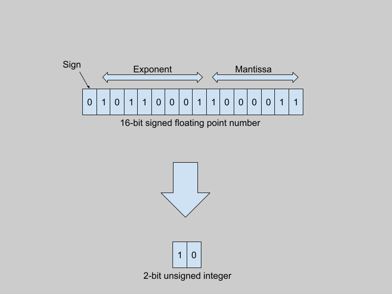
There are different ways to represent real numbers in computer systems, such as 32-bit floating point numbers, 8-bit integers, and so on. Regardless of the representation, computers can only express numbers in a finite range and of a limited precision. 32-bit floating point numbers (using the IEEE 754 32-bit base-2 system) have a range from -3.4 * 10³⁸ to +3.4 * 10³⁸. The smallest positive number that can be encoded in this format is of the order of 1 * 10^-38. In contrast, signed 8-bit integers range from -128 to +127.
Traditionally, model weights are represented as 32-bit floats (or as 16-bit floats, in the case of many large models). When quantized to 8-bit integers (for example), the quantizer function maps the entire range of 32-bit floating point numbers to integers between -128 and +127.
Scaling Number Ranges
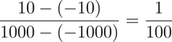
Consider a rudimentary example: you need to map numbers in the integer range A from -1000 to 1000 to the integer range B from -10 to +10. Intuitively, the number 500 in range A maps to the number 5 in range B. The steps below illustrate how to do this formulaically:
To transform a number from one range to another, you need to multiply it by the right scaling factor. The number 500 from range A can be expressed in the range B as follows:
500 * scaling_factor = Representation of 500 in Range B = 5
To calculate the scaling factor, take the ratio of the difference between the maximum and minimum values of the target range to the original range:
To map the number 500, multiply it by the scaling factor:
500 * (1/100) = 5
Based on the above formulation, try to map the number 510:
510 * (1/100) = 5.1
Since the range B consists only of integers, extend the above formula with a rounding function:
Round ( 510 * (1/100) ) = 5
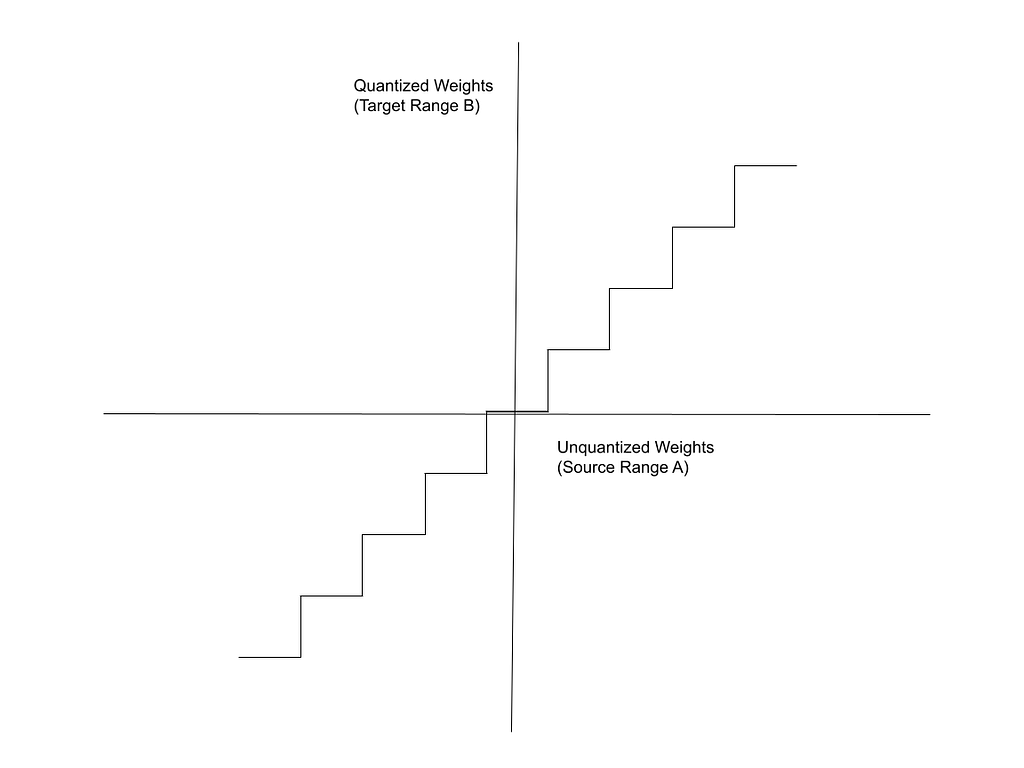
Similarly, all the numbers from 500 to 550 in Range A map to the number 5 in Range B. Based on this, notice that the mapping function resembles a step function with uniform steps.
Image created by author
The X-axis in this figure represents the source Range, A (unquantized weights) and the Y-axis represents the target Range, B (quantized weights).
Simple Integer Quantization
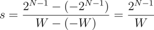
As a more practical example, consider a floating point range -W to +W, which you want to quantize to signed N-bit integers. The range of signed N-bit integers is -2^(N-1) to +2^(N-1)-1. But, to simplify things for the sake of illustration, assume a range from -2^(N-1) to +2^(N-1). For example, (signed) 8-bit integers range from -16 to +15 but here we assume a range from -16 to +16. This range is symmetric around 0 and the technique is called symmetric range mapping.
The scaling factor, s, is:
The quantized number is the product of the unquantized number and the scaling factor. To quantize to integers, we need to round this product to the nearest integer:
To remove the assumption that the target range is symmetric around 0, you also account for the zero-point offset, as explained in the next section.
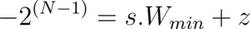
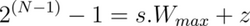
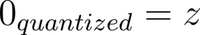
Zero Point Quantization
The number range -2^(N-1) to +2^(N-1), used in the previous example, is symmetric around 0. The range -2^(N-1) to +2^(N-1)-1, represented by N-bit integers, is not symmetric.
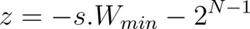
When the quantization number range is not symmetric, you add a correction, called a zero point offset, to the product of the weight and the scaling factor. This offset shifts the range such that it is effectively symmetric around zero. Conversely, the offset represents the quantized value of the number 0 in the unquantized range. The steps below show how to calculate the zero point offset, z.
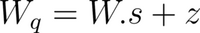
The quantization relation with the offset is expressed as:
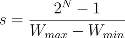
Map the extreme points of the original and the quantized intervals. In this context, W_min and W_max refer to the minimum and maximum weights in the original unquantized range.
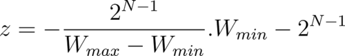
Solving these linear equations for the scaling factor, s, we get:
Similarly, we can express the offset, z, in terms of scaling factor s, as:
Substituting for s in the above relation:
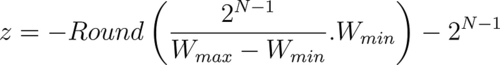
Since we are converting from floats to integers, the offset also needs to be an integer. Rounding the above expression:
Meaning of Zero-Point
In the above discussion, the offset value is called the zero-point offset. It is called the zero-point because it is the quantized value of the floating point weight of 0.
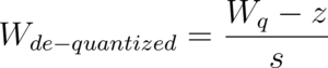
The function to obtain an approximation of the original floating point value from the quantized value is called the de-quantization function. It is simply the inverse of the original quantization relation:
Ideally, the de-quantized weight should be equal to the original weight. But, because of the rounding operations in the quantization functions, this is not the case. Thus, there is a loss of information involved in the de-quantization process.
Improving the Precision of Quantization
The biggest drawback of the above methods is the loss of precision. Bhandare et al, in a 2019 paper titled Efficient 8-Bit Quantization of Transformer Neural Machine Language Translation Model, were the first to quantize Transformer models. They demonstrated that naive quantization, as discussed in earlier sections, results in a loss of precision. In gradient descent, or indeed any optimization algorithm, the weights undergo just a slight modification in each pass. It is therefore important for the quantization method to be able to capture fractional changes in the weights.
Clipping the Range
Quantized intervals have a fixed and limited range of integers. On the other hand, unquantized floating points have a very large range. To increase the precision, it is helpful to reduce (clip) the range of the floating point interval.
It is observed that the weights in a neural network follow a statistical distribution, such as a normal Gaussian distribution. This means, most of the weights fall within a narrow interval, say between W_max and W_min. Beyond W_max and W_min, there are only a few outliers.
In the following description, the weights are clipped, and W_max and W_min refer to the maximum and minimum values of the weights in the clipped range.
Clipping (restricting) the range of the floating point weights to this interval means:
Weights which fall in the tails of the distribution are clipped — Weights higher than W_max are clipped to W_max. Weights smaller than W_min are clipped to W_min. The range between W_min and W_max is the clipping range.
Because the range of the floating point weights is reduced, a smaller unquantized range maps to the same quantized range. Thus, the quantized range can now account for smaller changes in the values of the unquantized weights.
The quantization formula shown in the previous section is modified to include the clipping:
The clipping range is customizable. You can choose how narrow you want this interval to be. If the clipping is overly aggressive, weights that contribute to the model’s accuracy can be lost in the clipping process. Thus, there is a tradeoff — clipping to a very narrow interval increases the precision of the quantization of weights within the interval, but it also reduces the model’s accuracy due to loss of information from those weights which were considered as outliers and got clipped.
Determining the Clipping Parameters
It has been noted by many researchers that the statistical distribution of model weights has a significant effect on the model’s performance. Thus, it is essential to quantize weights in such a way that these statistical properties are preserved through the quantization. Using statistical methods, such as Kullback Leibler Divergence, it is possible to measure the similarity of the distribution of weights in the quantized and unquantized distributions.
The optimal clipped values of W_max and W_min are chosen by iteratively trying different values and measuring the difference between the histograms of the quantized and unquantized weights. This is called calibrating the quantization. Other approaches include minimizing the mean square error between the quantized weights and the full-precision weights.
Different Scaling Factors
There is more than one way to scale floating point numbers to lower precision integers. There are no hard rules on what is the right scaling factor. Researchers have experimented with various approaches. A general guideline is to choose a scaling factor so that the unquantized and quantized distributions have a similar statistical properties.
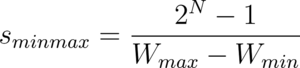
MinMax Quantization
The examples in the previous sections scale each weight by the difference of W_max and W_min (the maximum and minimum weights in the set). This is known as minmax quantization.
This is one of the most common approaches to quantization.
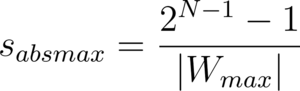
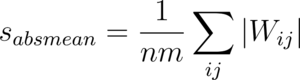
AbsMax Quantization
It is also possible to scale the weights by the absolute value of the maximum weight:
It is possible to quantize all the weights in a model using the same quantization scale. However, for better accuracy, it is also common to calibrate and estimate the range and quantization formula separately for each tensor, channel, and layer. The article Different Approaches to Quantization discusses the granularity levels at which quantization is applied.
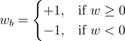
Extreme Quantization
Traditional quantization approaches reduce the precision of model weights to 16-bit or 8-bit integers. Extreme quantization refers to quantizing weights to 1-bit and 2-bit integers. Quantization to 1-bit integers ({0, 1}) is called binarization. The simple approach to binarize floating point weights is to map positive weights to +1 and negative weights to -1:
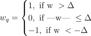
Similarly, it is also possible to quantize weights to ternary ({-1, 0, +1}):
In the above system, Delta is a threshold value. In a simplistic approach, one might quantize to ternary as follows:
Normalize the unquantized weights to lie between -1 and +1
Quantize weights below -0.5 to -1
Quantize weights between -0.5 and +0.5 to 0
Quantize weights above 0.5 to +1.
Directly applying binary and ternary quantization leads to poor results. As discussed earlier, the quantization process must preserve the statistical properties of the distribution of the model weights. In practice, it is common to adjust the range of the raw weights before applying the quantization and to experiment with different scaling factors.
The premise of binarization is that even though this process (binarization) seems to result in a loss of information, using a large number of weights compensates for this loss. The statistical distribution of the binarized weights is similar to that of the unquantized weights. Thus, deep neural networks are still able to demonstrate good performance even with binary weights.
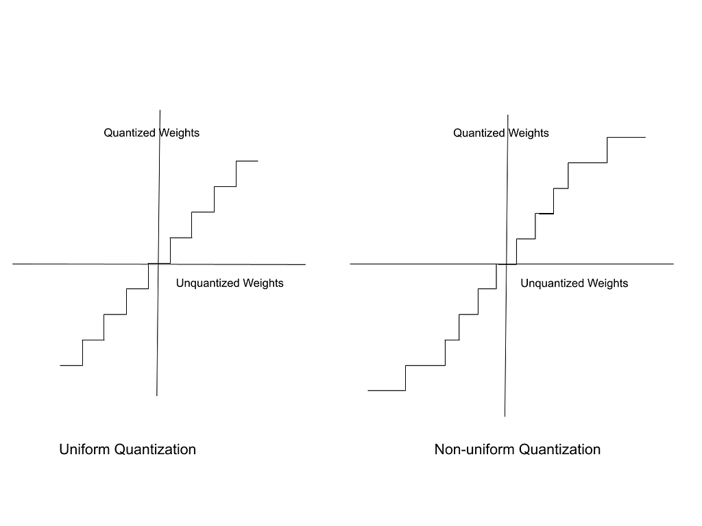
Non-uniform Quantization
The quantization methods discussed so far uniformly map the range of unquantized weights to quantized weights. They are called “uniform” because the mapping intervals are equidistant. To clarify, when you mapped the range -1000 to +1000 to the range -10 to +10:
All the numbers from -1000 to -951 are mapped to -10
The interval from -950 to -851 is mapped to -9
The interval from -850 to -751 maps to -8
and so on…
These intervals are also called bins.
The disadvantage of uniform quantization is that it does not take into consideration the statistical distribution of the weights themselves. It works best when the weights are equally distributed between W_max and W_min. The range of floating point weights can be considered as divided into uniform bins. Each bin maps to one quantized weight.
In reality, floating point weights are not distributed uniformly. Some bins contain a large number of unquantized weights while other bins have very few. Non-uniform quantization aims to create these bins in such a way that bins with a higher density of weights map to a larger interval of quantized weights.
There are different ways of representing the non-uniform distribution of weights, such as K-means clustering. However, these methods are not currently used in practice, due to the computational complexity of their implementation. Most practical quantization systems are based on uniform quantization.
In the hypothetical graph below, in the chart on the right, unquantized weights have a low density of distribution towards the edges and a high density around the middle of the range. Thus, the quantized intervals are larger towards the edges and compact in the middle.
Image created by author
Quantizing Activations and Biases
The activation is quantized similarly as the weights are, but using a different scale. In some cases, the activation is quantized to a higher precision than the weights. In models like BinaryBERT, and the 1-bit Transformer — BitNet, the weights are quantized to binary but the activations are in 8-bit.
The biases are not always quantized. Since the bias term only undergoes a simple addition operation (as opposed to matrix multiplication), the computational advantage of quantizing the bias is not significant. Also, the number of bias terms is much less than the number of weights.
Conclusion
This article explained (with numerical examples) different commonly used ways of quantizing floating point model weights. The mathematical relationships discussed here form the foundation of quantization to 1-bit weights and to 1.58-bit weights — these topics are discussed later in the series.
To learn more about the mathematical principles of quantization, refer to this 2023 survey paper by Weng. Quantization for Neural Networks by Lei Mao explains in greater detail the mathematical relations involved in quantized neural networks, including non-linear activation functions like the ReLU. It also has code samples implementing quantization. The next article in this series, Quantizing Neural Network Models, presents the high-level processes by which neural network models are quantized.
We use cookies on our website to give you the most relevant experience by remembering your preferences and repeat visits. By clicking “Accept”, you consent to the use of ALL the cookies.
This website uses cookies to improve your experience while you navigate through the website. Out of these, the cookies that are categorized as necessary are stored on your browser as they are essential for the working of basic functionalities of the website. We also use third-party cookies that help us analyze and understand how you use this website. These cookies will be stored in your browser only with your consent. You also have the option to opt-out of these cookies. But opting out of some of these cookies may affect your browsing experience.
Necessary cookies are absolutely essential for the website to function properly. These cookies ensure basic functionalities and security features of the website, anonymously.
Cookie
Duration
Description
cookielawinfo-checkbox-analytics
11 months
This cookie is set by GDPR Cookie Consent plugin. The cookie is used to store the user consent for the cookies in the category "Analytics".
cookielawinfo-checkbox-functional
11 months
The cookie is set by GDPR cookie consent to record the user consent for the cookies in the category "Functional".
cookielawinfo-checkbox-necessary
11 months
This cookie is set by GDPR Cookie Consent plugin. The cookies is used to store the user consent for the cookies in the category "Necessary".
cookielawinfo-checkbox-others
11 months
This cookie is set by GDPR Cookie Consent plugin. The cookie is used to store the user consent for the cookies in the category "Other.
cookielawinfo-checkbox-performance
11 months
This cookie is set by GDPR Cookie Consent plugin. The cookie is used to store the user consent for the cookies in the category "Performance".
viewed_cookie_policy
11 months
The cookie is set by the GDPR Cookie Consent plugin and is used to store whether or not user has consented to the use of cookies. It does not store any personal data.
Functional cookies help to perform certain functionalities like sharing the content of the website on social media platforms, collect feedbacks, and other third-party features.
Performance cookies are used to understand and analyze the key performance indexes of the website which helps in delivering a better user experience for the visitors.
Analytical cookies are used to understand how visitors interact with the website. These cookies help provide information on metrics the number of visitors, bounce rate, traffic source, etc.
Advertisement cookies are used to provide visitors with relevant ads and marketing campaigns. These cookies track visitors across websites and collect information to provide customized ads.