Tag: artificial intelligence

How to solve the tension between exploitation and exploration, and making sure you have devoted users that are happy with your visualization tools.

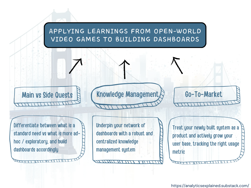
Developers of open world video games have a very interesting problem — how to allow and encourage the exploration of the world while at the same time making sure the players finish the main quests and follow a certain set of rules?

Analytics managers who are trying to enable their less savvy colleagues with dashboards know this exact same problem. They constantly face this tension between “exploration” and “exploitation”. On one hand, they need to build a system that is comprehensive enough to allow for the exploration of edge cases. On the other hand, they must not “drown” their users with too much information. Finding the right balance is often pretty complicated.

Let’s go back to our open-world video games developers. To make their games enjoyable while solving for the tension between exploration and exploitation, they:

(1) Build one main storyline, with alternative paths (i.e. “side quests”)

(2) Include a robust knowledge management system:

• They offer “an adventure log” where you can keep track of key informations
• They often start with a tutorial

(3) Power “online communities” and offer places for experts to share their knowledge

(4) Patch things and improve game mechanics over time

A strategy that can also be applied by analytics managers.

What are your users’ main quests?

Imagine: You’re a salesperson and you’re trying to understand how much money the customer you’re meeting with in a few minutes has been spending with your company in the past 2 years. You try to pull up a dashboard on your mobile phone — it doesn’t have mobile support. You try to resize the screen to find the right filters to use — your customer has multiple business locations so you need to filter by them all. Then the dashboard takes 2 minutes to load the last 6 months, but you actually needed the last 2 years and you forgot to update the filter for that..

There is a high chance that at some point, you gave up and just messaged your data analyst friend.

In the example above — being able to get relevant data about their portfolio in a matter of minutes is a “standard” need for salespeople — meaning that it is a repeated need that most of them have as part of their usual process / workflow. It is basically part of their main quest.

Zooming out: each team has a set of metrics they need to track on a regular basis and with a pre-defined granularity. For those metrics, they need dashboards that are simple to use, with a limited number of metrics and filters.

Once they have those dashboards in place that fulfill their primary needs effectively, they will start making feature requests for some additions (“ah, it would be nice if we could also see X,Y,Z”). Before you add these requests to existing dashboards, it is important to keep a first-principle approach: what use case was this dashboard supposed to fulfill?

From experience, it is better to:

1. Have one centralized dashboard for standard use cases — that is pretty limited in terms of metrics and filters.
2. Have one (or several) dashboards solving for edge cases as well as allowing the team to do some exploration.

Beware of dashboard inflation though as that can create a lot of issues down the line (from maintenance to conflicting data). It is important to always keep track of which dashboard is solving which use cases — and make sure what can be consolidated is consolidated. Your “dashboard ecosystem” (i.e. your suite of dashboards) will thrive only if you have a holistic approach and you make sure that each of your tools are differentiated and don’t overlap.

And with this approach, you can solve ~50% of the most common issues that are reported regarding dashboards, and your dashboards can effectively start complementing and simplifying your users’ routines (instead of complicating them).

Supporting your dashboard ecosystem with a robust knowledge management system

Your newly formed system can only be successful if people understand it and start using it. For the former, building a robust knowledge management system (KMS) is key. This KMS ensures everyone can find the relevant info re:your dashboards: where they are, what info they contain, what data transformations are being done, etc. An effective Knowledge Management System is:

• Centralized: In one single location
• Current: Regularly updated with the latest info
• Searchable: Allowing team members to easily locate the content they need.
• Always Improving: With a strong feedback loop
• Discoverable: People know about the KMS / how to find it

On top of establishing this KMS — you’ll want to conduct training sessions. Similar to tutorials in open-world games — where you learn how to use your weapons and fight battles — this is where you explain to your users how to win. A few tips:

• Try diverse learning formats: Some people will prefer instructor-led sessions, some will prefer self-service options — see what works best for your users and their schedule.
• Have a structured onboarding: Offer onboarding sessions for new users
• Offer practical exercises: Doing something in practice > Knowing something in theory, so try to include hands-on practice and real-world scenarios in these sessions.

With the above — you ensure that your team is not only equipped with powerful dashboards but also has the knowledge and training to use them effectively.

Track the usage of your ecosystem, and improve what needs to be improved

This step is often overlooked, but basically, you can’t generate value to your users if they never heard of your tool. Understanding how your users find your dashboards, what is your activation / retention rate for the different elements, where the drops in the funnel are, and how you can improve those are part to building a healthy ecosystem.

A few strategies that worked well for me are:

• Understanding and increasing activation: An “activated” user is a user that got sufficient value from your dashboards so that they keep using it in the future (aka become retained). Usually, activation can be achieved by offering extremely quick wins to your users within seconds of opening the dashboard.
• Building communities: Identify and nurture ‘super users’ in different teams. These individuals can act as advocates for the dashboard, offer peer-to-peer assistance and drive its usage within their networks.
• Actively gathering feedback and updating frequently: You are building this ecosystem for your users — so make sure you collect and act on user feedback. Surveys, suggestion boxes, and open channels for conversation ensure that the dashboard evolves in response to user needs.
• Communicating, again and again: While an email announcement is a good start, it’s just one lever in a larger strategy. The launch is only the beginning — try to send regular emails with updates, success stories on how people used the dashboards, plans, etc.

With those strategies, you ensure adoption and that your users will work with you — to build the best ecosystem that will generate the most value for them.

In conclusion..

A dashboard ecosystem success is as much about the “WHAT” than it is about the “HOW”. You can build the best tools in the world, but if your users don’t know about them, or if they don’t know how to use them — then they will never generate any value.

Hope you enjoyed reading this piece! Do you have any tips you’d want to share? Let everyone know in the comment section!

And If you want to read more of me, here are a few other articles you might like:

• How to Build a Successful Dashboard
• Building Analytically Mature Organizations (AMO)
• What Sets Great Data Analysts Apart

PS: This article was cross-posted to Analytics Explained, a newsletter where I distill what I learned at various analytical roles (from Singaporean startups to SF big tech), and answer reader questions about analytics, growth, and career.

---

Having a Comprehensive Dashboard Strategy for Analytics Managers was originally published in Towards Data Science on Medium, where people are continuing the conversation by highlighting and responding to this story.

Large Language Models, GPT-1 — Generative Pre-Trained Transformer

Diving deeply into the working structure of the first ever version of gigantic GPT-models

Introduction

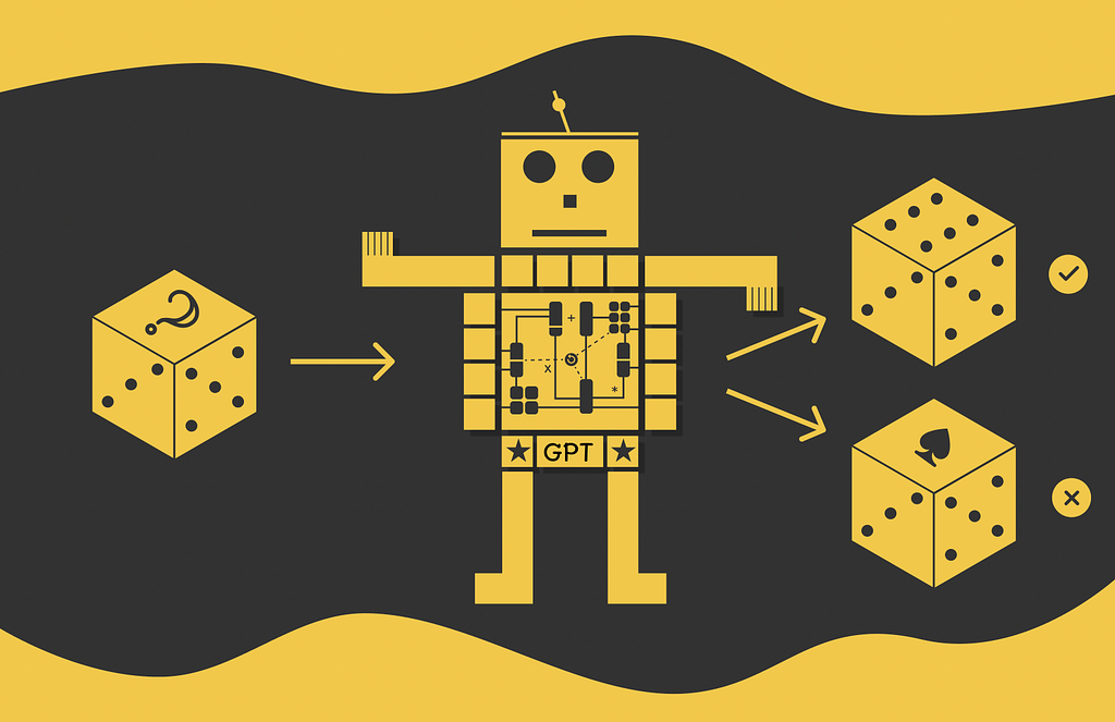
2017 was a historical year in machine learning. Researchers from the Google Brain team introduced Transformer which rapidly outperformed most of the existing approaches in deep learning. The famous attention mechanism became the key component in the future models derived from Transformer. The amazing fact about Transformer’s architecture is its vaste flexibility: it can be efficiently used for a variety of machine learning task types including NLP, image and video processing problems.

The original Transformer can be decomposed into two parts which are called encoder and decoder. As the name suggests, the goal of the encoder is to encode an input sequence in the form of a vector of numbers — a low-level format that is understood by machines. On the other hand, the decoder takes the encoded sequence and by applying a language modeling task, it generates a new sequence.

Encoders and decoders can be used individually for specific tasks. The two most famous models deriving their parts from the original Transformer are called BERT (Bidirectional Encoder Representations from Transformer) consisting of encoder blocks and GPT (Generative Pre-Trained Transformer) composed of decoder blocks.

In this article, we will talk about GPT and understand how it works. From the high-level perspective, it is necessary to understand that GPT architecture consists of a set of Transformer blocks as illustrated in the diagram above except for the fact that it does not have any input encoders.

Large Language Models: BERT — Bidirectional Encoder Representations from Transformer

Framework

As for most LLMs, GPT’s framework consists of two stages: pre-training and fine-tuning. Let us study how they are organised.

1. Pre-training

Loss function

As the paper states, “We use a standard language modeling objective to maximize the following likelihood”:

In this formula, at each step, the model outputs the probability distribution of all possible tokens being the next token i for the sequence consisting of the last k context tokens. Then, the logarithm of the probability for the real token is calculated and used as one of several values in the sum above for the loss function.

The parameter k is called the context window size.

The mentioned loss function is also known as log-likelihood.

Encoder models (e.g. BERT) predict tokens based on the context from both sides while decoder models (e.g. GPT) only use the previous context, otherwise they would not be able to learn to generate text.

The intuition behind the loss function

Since the expression for the log-likelihood might not be easy to comprehend, this section will explain in detail how it works.

As the name suggests, GPT is a generative model indicating that its ultimate goal is to generate a new sequence during inference. To achieve it, during training an input sequence is embedded and split by several substrings of equal size k. After that, for each substring, the model is asked to predict the next token by generating the output probability distribution (by using the final softmax layer) built for all vocabulary tokens. Each token in this distribution is mapped to the probability that exactly this token is the true next token in the subsequence.

To make the things more clear, let us look at the example below in which we are given the following string:

We split this string into substrings of length k = 3. For each of these substrings, the model outputs a probability distribution for the language modeling task. The predicted distrubitons are shown in the table below:

In each distribution, the probability corresponding to the true token in the sequence is taken (highlighted in yellow) and used for loss calculation. The final loss equals the sum of logarithms of true token probabilities.

GPT tries to maximise its loss, thus higher loss values correspond to better algorithm performance.

From the example distributions above, it is clear that high predicted probabilities corresponding to true tokens add up larger values to the loss function demonstrating better performance of the algorithm.

Subtlety behind the loss function

We have understood the intuition behind the GPT’s pre-training loss function. Nevertheless, the expression for the log-likelihood was originally derived from another formula and could be much easier to interpret!

Let us assume that the model performs the same language modeling task. However, this time, the loss function will maximize the product of all predicted probabilities. It is a reasonable choice as all of the output predicted probabilities for different subsequences are independent.

Since probability is defined in the range [0, 1], this loss function will also take values in that range. The highest value of 1 indicates that the model with 100% confidence predicted all the corrected tokens, thus it can fully restore the whole sequence. Therefore,

Product of probabilities as the loss function for a language modeling task, maximizes the probability of correctly restoring the whole sequence(-s).

If this loss function is so simple and seems to have such a nice interpretation, why it is not used in GPT and other LLMs? The problem comes up with computation limits:

• In the formula, a set of probabilities is multiplied. The values they represent are usually very low and close to 0, especially when during the beginning of the pre-training step when the algoroithm has not learned anything yet, thus assigning random probabilities to its tokens.
• In real life, models are trained in batches and not on single examples. This means that the total number of probabilities in the loss expression can be very high.

As a consequence, a lot of tiny values are multiplied. Unfortunately, computer machines with their floating-point arithmetics are not good enough to precisely compute such expressions. That is why the loss function is slightly transformed by inserting a logarithm behind the whole product. The reasoning behind doing it is two useful logarithm properties:

• Logarithm is monotonic. This means that higher loss will still correspond to better performance and lower loss will correspond to worse performance. Therefore, maximizing L or log(L) does not require modifications in the algorithm.

• The logarithm of a product is equal to the sum of the logarithms of its factors, i.e. log(ab) = log(a) + log(b). This rule can be used to decompose the product of probabilities into the sum of logarithms:

We can notice that just by introducing the logarithmic transformation we have obtained the same formula used for the original loss function in GPT! Given that and the above observations, we can conclude an important fact:

The log-likelihood loss function in GPT maximizes the logarithm of the probability of correctly predicting all the tokens in the input sequence.

Text generation

Once GPT is pre-trained, it can already be used for text generation. GPT is an autoregressive model meaning that it uses previously predicted tokens as input for prediction of next tokens.

On each iteration, GPT takes an initial sequence and predicts the next most probable token for it. After that, the sequence and the predicted token are concatenated and passed as input to again predict the next token, etc. The process lasts until the [end] token is predicted or the maximum input size is reached.

2. Fine-tuning

After pre-training, GPT can capture linguistic knowledge of input sequences. However, to make it better perform on downstream tasks, it needs to be fine-tuned on a supervised problem.

For fine-tuning, GPT accepts a labelled dataset where each example contains an input sequence x with a corresponding label y which needs to be predicted. Every example is passed through the model which outputs their hidden representations h on the last layer. The resulting vectors are then passed to an added linear layer with learnable parameters W and then through the softmax layer.

The loss function used for fine-tuning is very similar to the one mentioned in the pre-training phase but this time, it evaluates the probability of observing the target value y instead of predicting the next token. Ultimately, the evaluation is done for several examples in the batch for which the log-likelihood is then calculated.

Additionally, the authors of the paper found it useful to include an auxiliary objective used for pre-training in the fine-tuning loss function as well. According to them, it:

• improves the model’s generalization;
• accelerates convergence.

Finally, the fine-tuning loss function takes the following form (α is a weight):

Input format on downstream tasks

There exist a lot of approaches in NLP for fine-tuning a model. Some of them require changes in the model’s architecture. The obvious downside of this methodology is that it becomes much harder to use transfer learning. Furthermore, such a technique also requires a lot of customizations to be made for the model which is not practical at all.

On the other hand, GPT uses a traversal-style approach: for different downstream tasks, GPT does not require changes in its architecture but only in the input format. The original paper demonstrates visualised examples of input formats accepted by GPT on various downstream problems. Let us separately go through them.

Classification

This is the simplest downstream task. The input sequence is wrapped with [start] and [end] tokens (which are trainable) and then passed to GPT.

Textual entailment

Textual entailment or natural language inference (NLI) is a problem of determining whether the first sentence (premise) is logically followed by the second (hypothesis) or not. For modeling that task, premise and hypothesis are concatenated and separated by a delimiter token ($).

Semantic similarity

The goal of similarity tasks is to understand how semantically close a pair of sentences are to each other. Normally, compared pairs sentences do not have any order. Taking that into account, the authors propose concatenating pairs of sentences in both possible orders and feeding the resulting sequences to GPT. The both hidden output Transformer layers are then added element-wise and passed to the final linear layer.

Question answering & Multiple choice answering

Multiple choice answering is a task of correctly choosing one or several answers to a given question based on the provided context information.

For GPT, each possible answer is concatenated with the context and the question. All the concatenated strings are then independently passed to Transformer whose outputs from the Linear layer are then aggregated and final predictions are chosen based on the resulting answer probability distribution.

Setup

GPT is pre-trained on the BookCorpus dataset containing 7k books. This dataset was chosen on purpose since it mostly consists of long stretches of text allowing the model to better capture language information on a long distance. Speaking of architecture and training details, the model has the following parameters:

• Number of Transformer blocks: 12
• Embedding size: 768
• Number of attention heads: 12
• FFN hidden state size: 3072
• Optimizator: Adam (learning rate is set to 2.5e-4)
• Activation function: GELU
• Byte-pair encoding with a vocabulary size of 40k is used
• Total number of parameters: 120M

Finally, GPT is pre-trained on 100 epochs tokens with a batch size of 64 on continuous sequences of 512 tokens.

Most of hyperparameters used for fine-tuning are the same as those used during pre-training. Nevertheless, for fine-tuning, the learning rate is decreased to 6.25e-5 with the batch size set to 32. In most cases, 3 fine-tuning epochs were enough for the model to produce strong performance.

Byte-pair encoding helps deal with unknown tokens: it iteratively constructs vocabulary on a subword level meaning that any unknown token can be then split into a combination of learned subword representations.

Conclusion

Combination of the power of Transformer blocks and elegant architecture design, GPT has become one of the most fundamental models in machine learning. It has established 9 out of 12 new state-of-the-art results on top benchmarks and has become a crucial foundation for its future gigantic successors: GPT-2, GPT-3, GPT-4, ChatGPT, etc.

Resources

• Improving Language Understanding by Generative Pre-Training

All images are by the author unless noted otherwise

---

Large Language Models, GPT-1 — Generative Pre-Trained Transformer was originally published in Towards Data Science on Medium, where people are continuing the conversation by highlighting and responding to this story.

Everything you need to know about how context windows affect Transformer training and usage

The context window is the maximum sequence length that a transformer can process at a time. With the rise of proprietary LLMs that limit the number of tokens and therefore the prompt size — as well as the growing interest in techniques such as Retrieval Augmented Generation (RAG)— understanding the key ideas around context windows and their implications is becoming increasingly important, as this is often cited when discussing different models.

The transformer architecture is a powerful tool for natural language processing, but it has some limitations when it comes to handling long sequences of text. In this article, we will explore how different factors affect the maximum context length that a transformer model can process, and whether bigger is always better when choosing a model for your task.

How many words can I fit into a Transformer?

At the time of writing, models such as the Llama-2 variants have a context length of 4k tokens, GPT-4 turbo has 128k, and Claude 2.1 has 200k! From the number of tokens alone, it can be difficult to envisage how this translates into words; whilst it depends on the tokenizer used, a good rule of thumb is that 100k tokens is approximately 75,000 words. To put that in perspective, we can compare this to some popular literature:

• The Lord of the Rings (J. R. R. Tolkien): 564,187 words, 752k tokens
• Dracula (Bram Stoker): 165,453 words, 220k tokens
• Grimms’ Fairy Tales (Jacob Grimm and Wilhelm Grimm): 104,228 words, 139k tokens
• Frankenstein (Mary Shelley): 78,100 words, 104k tokens
• Harry Potter and the Philosopher’s Stone (J. K. Rowling): 77,423 words, 103k tokens
• Treasure Island (Robert Louis Stevenson): 72,036 words, 96k tokens
• The War of the Worlds (H. G. Wells): 63,194 words, 84k tokens
• The Hound of the Baskervilles (Arthur Conan Doyle): 62,297 words, 83k tokens
• The Jungle Book (Rudyard Kipling): 54,178 words, 72k tokens

To summarise, 100k tokens is roughly equivalent to a short novel, whereas at 200k we can almost fit the entirety of Dracula, a medium sized volume! To ingest a large volume, such as The Lord of the Rings, we would need 6 requests to GPT-4 and only 4 calls to Claude 2!

What determines the size of the context window?

At this point, you may be wondering why some models have larger context windows than others.

To understand this, let’s first review how the attention mechanism works in the figure below; if you aren’t familiar with the details of attention, this is covered in detail in my previous article. Recently, there have been several attention improvements and variants which aim to make this mechanism more efficient, but the key challenges remain the same. Here, will focus on the original scaled dot-product attention.

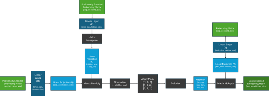
From the figure above, we can notice that the size of the matrix containing our attention scores is determined by the lengths of the sequences passed into the model and can grow arbitrarily large! Therefore, we can see that the context window is not determined by the architecture, but rather the length of the sequences that are given to the model during training.

This calculation can be incredibly expensive to compute as, without any optimisations, matrix multiplications are generally quadratic in space complexity (O(n^2)). Put simply, this means that if the length of an input sequence doubles, the amount of memory required quadruples! Therefore, training a model on sequence lengths of 128k will require approximately 1024 times the memory compared to training on sequence lengths of 4k!

It is also important to keep in mind that this operation is repeated for every layer and every head of the transformer, which results in a significant amount of computation. As the amount of GPU memory available is also shared with the parameters of the model, any computed gradients, and a reasonable sized batch of input data, hardware can quickly become a bottleneck on the size of the context window when training large models.

Can we extend the context window of a pre-trained model?

After understanding the computational challenges of training models on longer sequence lengths, it may be tempting to train a model on short sequences, with the hope that this will generalise to longer contexts.

One obstacle to this is the positional encoding mechanism, used to enable transformers to capture the position of tokens in a sequence. In the original paper, two strategies for positional encoding were proposed. The first was to use learnable embeddings specific to each position in the sequence, which are clearly unable to generalise past the maximum sequence length that the model was trained on. However, the authors hypothesised that their preferred sinusoidal approach may extrapolate to longer sequences; subsequent research has demonstrated that this is not the case.

In many recent transformer models such as PaLM and Llama-2, absolute positional encodings have been replaced by relative positional encodings, such as RoPE, which aim to preserve the relative distance between tokens after encodings. Whilst these are slightly better at generalising to longer sequences than previous approaches, performance quickly breaks down for sequence lengths significantly longer than the model has seen before.

Whilst there are several approaches that aim to change or remove positional encodings completely, these require fundamental changes to the transformer architecture, and would require models to be retrained, which is highly expensive and time consuming. As many of the top performing open-source models at the time of writing, are derived from pretrained versions of Llama-2, there is a lot of active research taking place into how to extend the context length of existing model which use RoPE embeddings, with varying success.

Many of these approaches employ some variation of interpolating the input sequence; scaling the positional embeddings so that they fit within the original context window of the model. The intuition behind this is that it should be easier for the model fill in the gaps between words, rather than trying to predict what comes after the words.

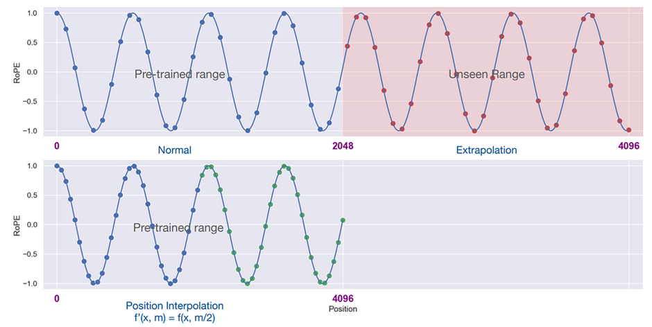
One such approach, known as YaRN, was able to extend the context window of the Llama-2 7B and 13B models to 128k without a significant degradation in performance!

Whilst a definitive approach that works well in all contexts has yet to emerge, this remains an exciting area of research, with big potential implications!

Are longer context windows always better?

Now that we understand some of the practical challenges around training models on longer sequence lengths, and some potential mitigations to overcome this, we can ask another question — is this extra effort worth it? At first glance, the answer may seem obvious; providing more information to a model should make it easier to inject new knowledge and reduce hallucinations, making it more useful in almost every conceivable application. However, things are not so simple.

In the 2023 paper Lost in the Middle, researchers at Stanford and Berkley investigated how models use and access information provided in their context window, and concluded the following:

“We find that changing the position of relevant information in the input context can substantially affect model performance, indicating that current language models do not robustly access and use information in long input contexts”.

For their experiments, the authors created a dataset where, for each query, they had a document that contains the answer and k — 1 distractor documents which did not contain the answer; adjusting the input context length by changing the number of retrieved documents that do not contain the answer. They then modulated the position of relevant information within the input context by changing the order of the documents to place the relevant document at the beginning, middle or end of the context, and evaluated whether any of the correct answers appear in the predicted output.

Specifically, they observed that the models studied performed the best when the relevant information was found at the start or the end of the context window; when the information required was in the middle of the context, performance significantly decreased.

In theory, the self-attention mechanism in a Transformer enables the model to consider all parts of the input when generating the next word, regardless of their position in the sequence. As such, I believe that any biases that the model has learned about where to find important information is more likely to come from the training data than the architecture. We can explore this idea further by examining the results that the authors observed when evaluating the Llama-2 family of models on the accuracy or retrieving documents based on their position, which are presented in the figure below.

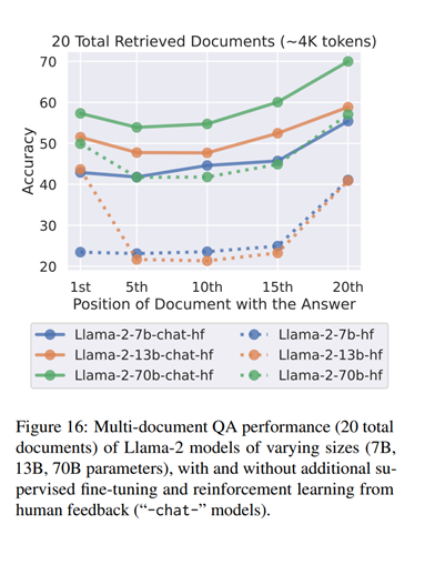
Looking at the base models, we can clearly observe the authors’ conclusions for the Llama-2 13B and 70B models. Interestingly, for the 7B model, we can see that it relies almost exclusively on the end of the context; as a lot of unsupervised finetuning is on streams of data scraped from various sources, when the model has relatively few parameters to dedicate to predicting the next word in an ever-changing context, it makes sense to focus on the most recent tokens!

The bigger models also perform well when the relevant information is at the beginning of the text; suggesting that they learn to focus more on the start of the text as they get more parameters. The authors hypothesise that this is because, during pre-training, the models see a lot of data from sources like StackOverflow which start with important information. I doubt the 13B model’s slight advantage with front-loaded information is significant, as the accuracy is similar in both cases and the 70B model does not show this pattern.

The ‘chat’ models are trained further with instruction tuning and RLHF, and they perform better overall, and also seem to become less sensitive to the position of the relevant information in the text. This is more clear for the 13B model, and less for the 70B model. The 7B model does not change much, perhaps because it has fewer parameters. This could mean that these models learn to use information from other parts of the text better after more training, but they still prefer the most recent information. Given that the subsequent training stages are significantly shorter, they have not completely overcome have the biases from the first unsupervised training; I suspect that the 70B model may require a larger, more diverse subsequent training to exhibit a similar magnitude of change as in the performance of the 13B model observed here.

Additionally, I would be interested in an investigation which explores the position of the relevant information in the text in the datasets used for SFT. As humans exhibit similar behaviour of being better at recalling information at the start and end of sequences, it would not be surprising if this behaviour is mirrored in a lot of the examples given.

Conclusion

To summarise, the context window is not fixed and can grow as large as you want it to, provided there is enough memory available! However, longer sequences mean more computation — which also result in the model being slower — and unless the model has been trained on sequences of a similar length, the output may not make much sense! However, even for models with large context windows, there is no guarantee that they will effectively use all of the information provided to them — there really is no free lunch!

Chris Hughes is on LinkedIn

Unless otherwise stated, all images were created by the author.

References

• RAG and generative AI — Azure AI Search | Microsoft Learn
• Llama 2 — Meta AI
• Models — OpenAI API
• Introducing Claude 2.1 Anthropic
• What are tokens and how to count them? | OpenAI Help Center
• De-coded: Transformers explained in plain English | by Chris Hughes | Towards Data Science
• [1706.03762] Attention Is All You Need (arxiv.org)
• Train Short, Test Long: Attention with Linear Biases enables input length extrapolation (openreview.net)
• [2203.16634] Transformer Language Models without Positional Encodings Still Learn Positional Information (arxiv.org)
• [2310.06825] Mistral 7B (arxiv.org)
• [2401.07872] The What, Why, and How of Context Length Extension Techniques in Large Language Models — A Detailed Survey (arxiv.org)
• [2306.15595] Extending Context Window of Large Language Models via Positional Interpolation (arxiv.org)
• [2309.00071] YaRN: Efficient Context Window Extension of Large Language Models (arxiv.org)
• [2307.03172] Lost in the Middle: How Language Models Use Long Contexts (arxiv.org)
• Primary Effect: Meaning, How It Works (verywellmind.com)
• No free lunch theorem — Wikipedia

---

De-Coded: Understanding Context Windows for Transformer Models was originally published in Towards Data Science on Medium, where people are continuing the conversation by highlighting and responding to this story.