Tag: artificial intelligence

Exploring mental well-being insights with zero-shot classification

Sentiment analysis is a powerful tool in natural language processing (NLP) for exploring public opinions and emotions in text. In the context of mental health, it can provide compelling insights into the holistic wellness of individuals. As a summer data science associate at The Rockefeller Foundation, I conducted a research project using NLP techniques to explore Reddit discussions on depression before and after the COVID-19 pandemic. In order to better understand gender-related taboos around mental health and depression, I chose to analyze the distinctions between posts made by men and women.

Different Types of Sentiment Analysis

Traditionally, sentiment analysis classifies the overall emotions expressed in a piece of text into three categories: positive, negative, or neutral. But what if you were interested in exploring emotions at a more granular level — such as anticipation, fear, sadness, anger, etc.

There are ways to do this using sentiment models that reference word libraries, like The NRC Emotion Lexicon, which associates texts with eight basic emotions (anger, fear, anticipation, trust, surprise, sadness, joy, and disgust). However, the setup for this kind of analysis can be complicated, and the tradeoff may not be worth it.

I found that zero-shot classification can easily be used to produce similar results. The term “zero-shot” comes from the concept that a model can classify data with zero prior exposure to the labels it is asked to classify. This eliminates the need for a training dataset, which is often time-consuming and resource-intensive to create. The model uses its general understanding of the relationships between words, phrases, and concepts to assign them into various categories.

I was able to repurpose the use of zero-shot classification models for sentiment analysis by supplying emotions as labels to classify anticipation, anger, disgust, fear, joy, and trust.

In this post, I’ll share how to quickly get started with sentiment analysis using zero-shot classification in 5 easy steps.

Platforms like HuggingFace simplify the implementation of these models. You can explore different models and test out the results to find which one to use by:

1. Go to https://huggingface.co
2. Click on the “Models” tab and select the type of NLP task you’re interested in
3. Choose one of the model cards, and this will lead you to the model interface
4. Pass in a string of text to see how the model performs

Here are a couple examples of how a sentiment analysis model performed compared to a zero-shot model.

Sentiment Analysis

These models classify text into negative, neutral, and positive categories.

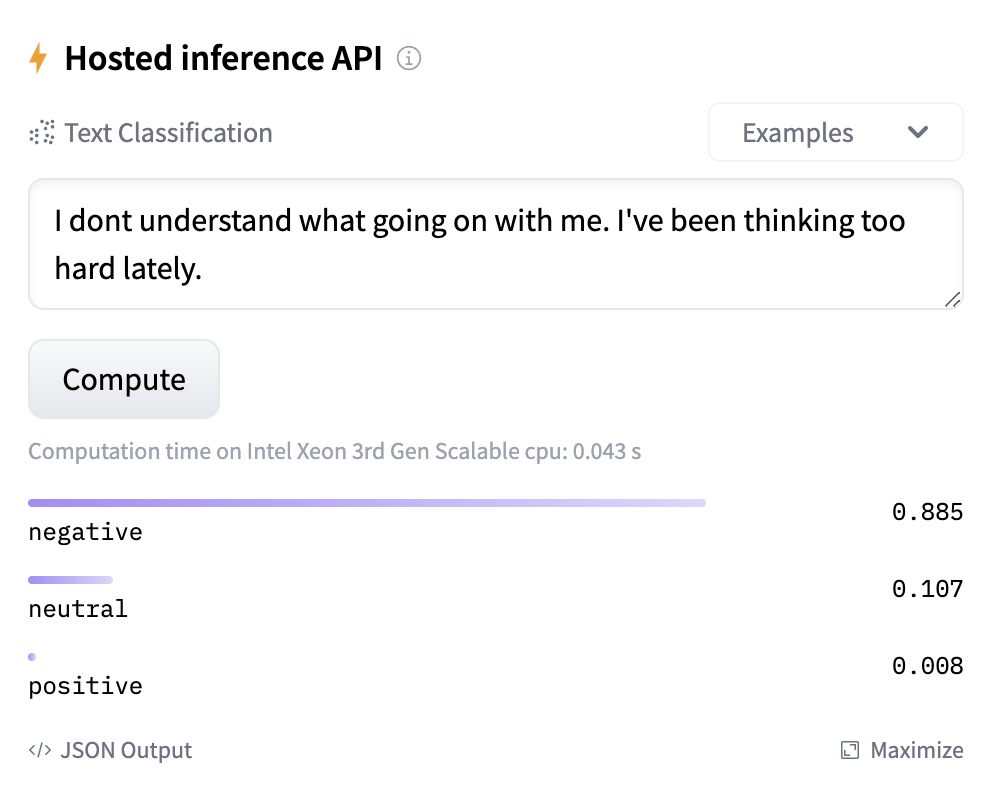
You can see here that the nuance is quite limited and does not leave a lot of room for interpretation. Access to the model shown above can be found here to test or run it.

These types of models are best used when you are looking to get a general pulse on the sentiment—whether the text is leaning positively or negatively.

Zero-shot classification

These models classify text into any categories you want by inputting them as labels. Since I was looking at text around mental health, I included emotions as labels, including urgent, joy, sadness, fatigue, and anxiety.

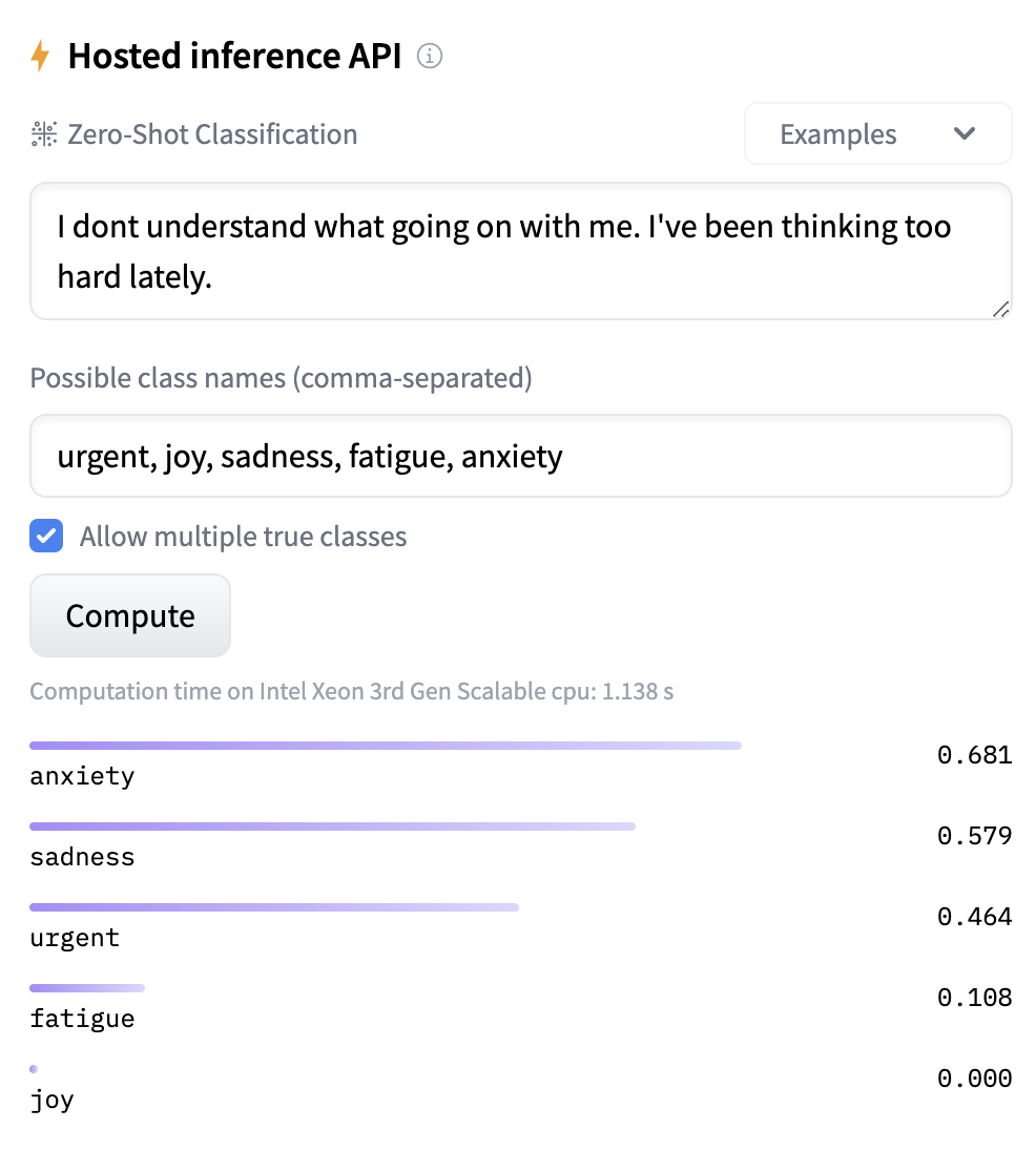
You can see that with the zero-shot classification model, we can easily categorize the text into a more comprehensive representation of human emotions without needing any labeled data. The model can discern nuances and changes in emotions within the text by providing accuracy scores for each label. This is useful in mental health applications, where emotions often exist on a spectrum.

Now that I have identified that the zero-shot classification model is a better fit for my needs, I will walk through how to apply the model to a dataset.

Implementation of the Zero-Shot Model

Here are the requirements to run this example:

torch>=1.9.0
transformers>=4.11.3 
datasets>=1.14.0 
tokenizers>=0.11.0
pandas
numpy

Step 1. Import libraries used

In this example, I am using the DeBERTa-v3-base-mnli-fever-anli zero-shot classifier from Hugging Face.

# load hugging face library and model


from transformers import pipeline
classifier = pipeline("zero-shot-classification", model="MoritzLaurer/DeBERTa-v3-base-mnli-fever-anli")

# load in pandas and numpy for data manipulation
import pandas as pd
import numpy as np

Pipeline is the function used to call in pre-trained models from HuggingFace. Here I am passing on two arguments. You can get the values for these arguments from the model card:

• `task`: The type of task the model is performing, passed as a string
• `model`: Name of the model you are using, passed as a string

Step 2. Read in your data

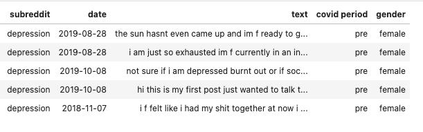
Your data can be in any form, as long as there is a text column where each row contains a string of text. To follow along with this example, you can read in the Reddit depression dataset here. This dataset is made available under the Public Domain Dedication and License v1.0.

#reading in data 
df = pd.read_csv("https://raw.githubusercontent.com/akaba09/redditmentalhealth/main/code/dep.csv")

Here is a preview of the dataset we’ll be using:

Step 3: Create a list of classes that you want to use for predicting sentiment

This list will be used as labels for the model to predict each piece of text. For example, is the text exploring emotions such as anger or disgust? In this case, I am passing a list of emotions as labels. You can use as many or as few labels as you’d like.

# Creating a list of emotions to use as labels
text_labels = ["anticipation", "anger", "disgust", "fear", "joy", "trust"]

Step 4: Run the model prediction on one piece of text first

Run the model on one piece of text first to understand what the model returns and how you want to shape it for your dataset.

# Sample piece of text
sample_text = "still have depression symptoms not as bad as they used to be in fact my therapist says im improving a lot but for the past years ive been stuck in this state of emotional numbness feeling disconnected from myself others and the world and time doesnt seem to be passing"

# Run the model on the sample text
classifier(sample_text, text_labels, multi_label = False)

The classifier function is part of the Transformers library in HuggingFace and calls in the model you want to use. In this example, we are using “DeBERTa-V4-base-mnli-fever-anli” and it takes three positional arguments:

• First position: a piece of text in string format. his variable can have any name. In this example, I named it `sample_text`
• Second position: list of labels you want to predict. This variable can have any name. In this example, I named it `text_labels`
• Third position: `multi_label` takes a true or false argument. This determines whether each piece of text can have multiple labels or only one label per text. In this example, I am only interested in one label per text.

Here’s the output you get from the sample text:

#output 
# {'sequence': ' still have depression symptoms not as bad as they used to be in fact my therapist says im improving a lot but for the past years ive been stuck in this state of emotional numbness feeling disconnected from myself others and the world and time doesnt seem to be passing',
 # 'labels': ['anticipation', 'trust', 'joy', 'disgust', 'fear', 'anger'],
 # 'scores': [0.6039842963218689,
   #0.1163715273141861,
   #0.074860118329525,
   #0.07247171550989151,
   #0.0699692890048027,
   #0.0623430535197258]}

The model returns a dictionary with the following keys and values”

• “sequence”: The piece of text we passed in
• “labels”: The list of labels for the model predictions in descending order of confidence.
• “scores”: This returns a list of scores that represent the model’s confidence in its predictions in descending order. The order is correlated to the labels, so the first element in the scores list is reflective of the first element in the labels list. In this example, the model has predicted “anticipation” with a 0.604 confidence level.

Step 5: Write a custom function to make predictions on the entire dataset and include the labels as part of the dataframe
Seeing the structure of the dictionary output from the model, I can write a custom function to apply the predictions to all my data. In this example, I am only interested in keeping one sentiment for each piece of text. This function will take in your dataframe and return a new dataframe that includes two new columns—one for your sentiment label and one for the model score.

def predict_sentiment(df, text_column, text_labels):
    
"""
    Predict the sentiment for a piece of text in a dataframe.

    Args:
        df (pandas.DataFrame): A DataFrame containing the text data to perform sentiment analysis on.
        text_column (str): The name of the column in the DataFrame that contains the text data.
        text_labels (list): A list of text labels for sentiment classification.

    Returns:
        pandas.DataFrame: A DataFrame containing the original data with additional columns for the predicted 
        sentiment label and corresponding score.

    Raises:
        ValueError: If the DataFrame (df) does not contain the specified text_column.

    Example:
        # Assuming df is a pandas DataFrame and text_labels is a list of text labels
        result = predict_sentiment(df, "text_column_name", text_labels)
    """
    
    result_list = []
    for index, row in df.iterrows():
        sequence_to_classify = row[text_column]
        result = classifier(sequence_to_classify, text_labels, multi_label = False)
        result['sentiment'] = result['labels'][0]
        result['score'] = result['scores'][0]
        result_list.append(result)
    result_df = pd.DataFrame(result_list)[['sequence','sentiment', 'score']]
    result_df = pd.merge(df, result_df, left_on = "text", right_on="sequence", how = "left")
    return result_df

This function iterates over your dataframe and parses the dictionary result for each row. Since I am only interested in the sentiment with the highest score, I am selecting the first label by indexing it into the list with result[‘labels’][0]. If you want to take the top three sentiments, for example, you can update with a range result[‘labels’][0:3]. Similarly, if you want the top three scores, you can update with a range result[‘scores’][0:3].

Now you can run the function on your dataframe!

# run prediction on df

results_df = predict_sentiment(df=df, text_column ="text", text_labels= text_labels)

Here I pass in three arguments:

• `df`: The name of your dataframe
• `text_column`: The name of the column in the dataframe that contains text. Pass this argument as a string.
• `text_labels`: A list of text labels for sentiment classification

This is a preview of what your returned data frame looks like:

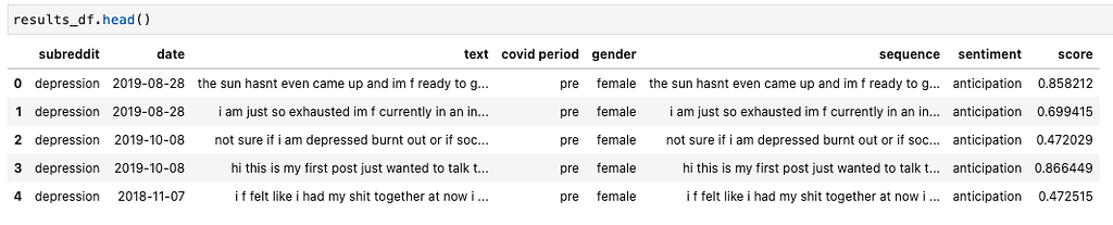
For each piece of text, you can get the associated sentiment along with the model score.

Conclusion

Classic sentiment analysis models explore positive or negative sentiment in a piece of text, which can be limiting when you want to explore more nuance, like emotions, in the text.

While you can explore emotions with sentiment analysis models, it usually requires a labeled dataset and more effort to implement. Zero-shot classification models are versatile and can generalize across a broad array of sentiments without needing labeled data or prior training.

As we explored in this example, zero-shot models take in a list of labels and return the predictions for a piece of text. We passed in a list of emotions as our labels, and the results were pretty good considering the model wasn’t trained on this type of emotional data. This type of classification is a valuable tool in analyzing mental health-related text, which allows us to gain a more comprehensive understanding of the emotional landscape and contributes to improved support for mental well-being.

All images, unless otherwise noted, are by the author.

Low, D. M., Rumker, L., Torous, J., Cecchi, G., Ghosh, S. S., & Talkar, T. (2020). Natural Language Processing Reveals Vulnerable Mental Health Support Groups and Heightened Health Anxiety on Reddit During COVID-19: Observational Study. Journal of medical Internet research, 22(10), e22635.

---

How to Use Zero-Shot Classification for Sentiment Analysis was originally published in Towards Data Science on Medium, where people are continuing the conversation by highlighting and responding to this story.

Getting Started Predicting Time Series Data with Facebook Prophet

This article aims to take away the entry barriers to get started with time series analysis in a hands-on tutorial using Prophet

When getting started with data science, time series analysis is a common thing people would love to try themselves! The general idea here is to learn from historical patterns over time to predict the future. Typical use cases could be weather predictions or sales forecasting. But what does all this have to do with this wise prophet below?!

This article aims to take away the entry barriers to get started with time series analysis in a hands-on tutorial using one of the easiest tools called Facebook Prophet within Google Colab (both are free!). In case you want to get started immediately, feel free to skip the next two chapters where I will give a short background on time series principles and also Facebook Prophet itself. Have fun!

This article is structured into three main sections:

#1 Brief introduction to Time Series Analysis principles
#2 An Introduction to Facebook Prophet
#3 Hands-on tutorial on how to use Prophet in Google Colab (for free)

#1 General Principles of Time Series Analysis

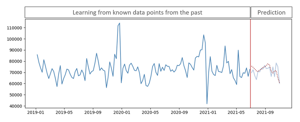
Imagine you are a store manager for consumer products and you want to predict the upcoming product demand to better manage the supply. A reasonable machine learning approach for this scenario is to run some time series analysis which involves understanding, modeling, and making predictions based on sequential data points. [1]

The below graphic illustrates an artificial development of historic product demand (dark-blue line) over time, which can be used to analyze a time series pattern. Our ultimate goal would be to predict (red-dotted line) the actual future demand (light-blue line) as precise as possible:

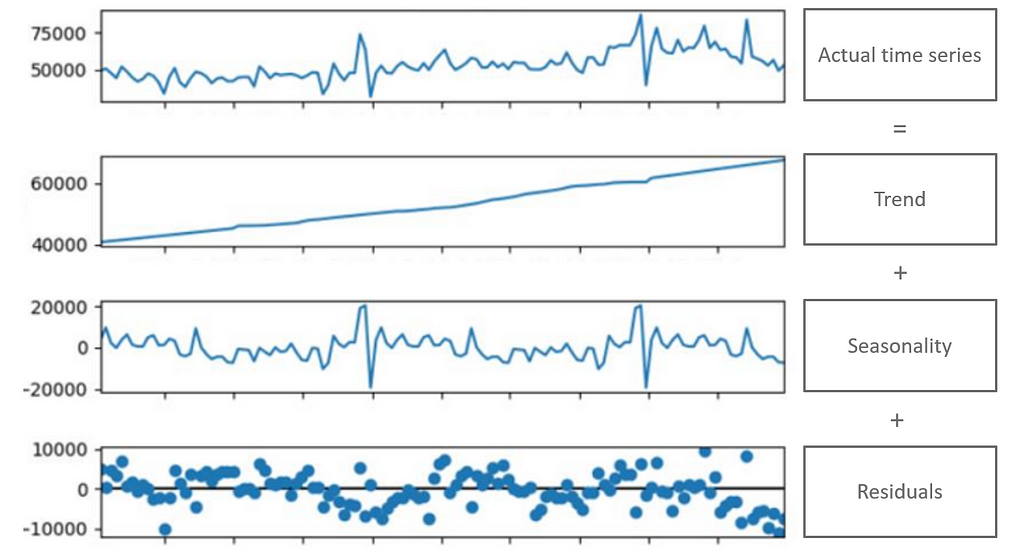
A time series is typically decomposed into three main components:

1. Trend: the long-term movement or general direction in the data.
2. Seasonality: fluctuations or patterns that repeat at regular intervals
3. Residual/error: remainder or leftover variation in the data

The decomposition of a time series into these three components, often referred to as additive or multiplicative decomposition, allows analysts to better understand the underlying structure and patterns. This understanding is essential for selecting appropriate forecasting models and making accurate predictions based on historical data. [2]

#2 What is Facebook Prophet?

Prophet is an open-source tool released by Facebook’s Data Science team that produces time series forecasting data based on an additive model where a non-linear trend fits with seasonality and holiday effects. The design principles allow parameter adjustments without much knowledge of the underlying model which makes the method applicable to teams with less statistical knowledge. [3]

Prophet is particularly well-suited for business forecasting applications, and it has gained popularity due to its ease of use and effectiveness in handling a wide range of time series data. As with every tool, keep in mind that while Prophet is powerful, the choice of forecasting method depends on the specific characteristics of the data and the goals of the analysis. In general, it is not granted that Prophet performs better than other models. However, Prophet comes with some useful features e.g., a reflection of seasonality change pre- and post-COVID or treating lockdowns as one-off holidays.

For a more in-depth introduction by Meta (Facebook) itself, look at the video below on YouTube.

In the following tutorial, we will implement and use Prophet with Python. However, you are more than happy to run your analysis using R as well!

#3 Hands-on tutorial on how to use Prophet

In case you have limited experience with or no access to your coding environment, I recommend making use of Google Colaboratory (“Colab”) which is somewhat like “a free Jupyter notebook environment that requires no setup and runs entirely in the cloud.” While this tutorial claims more about the simplicity and advantages of Colab, there are drawbacks as reduced computing power compared to proper cloud environments. However, I believe Colab might not be a bad service to take the first steps with Prophet.

To set up a basic environment for Time Series Analysis within Colab you can follow these two steps:

1. Open https://colab.research.google.com/ and register for a free account
2. Create a new notebook within Colab
3. Install & use the prophet package:

pip install prophet

from prophet import Prophet

Loading and preparing Data

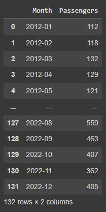
I uploaded a small dummy dataset representing the monthly amount of passengers for a local bus company (2012–2023). You can find the data here on GitHub.

As the first step, we will load the data using pandas and create two separate datasets: a training subset with the years 2012 to 2022 as well as a test subset with the year 2023. We will train our time series model with the first subset and aim to predict the passenger amount for 2023. With the second subset, we will be able to validate the accuracy later.

import pandas as pd

df_data = pd.read_csv("https://raw.githubusercontent.com/jonasdieckmann/prophet_tutorial/main/passengers.csv")

df_data_train = df_data[df_data["Month"] < "2023-01"]
df_data_test = df_data[df_data["Month"] >= "2023-01"]

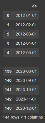
display(df_data_train)

The output for the display command can be seen below. The dataset contains two columns: the indication of the year-month combination as well as a numeric column with the passenger amount in that month. Per default, Prophet is designed to work with daily (or even hourly) data, but we will make sure that the monthly pattern can be used as well.

Decomposing training data

To get a better understanding of the time series components within our dummy data, we will run a quick decomposing. For that, we import the method from statsmodels library and run the decomposing on our dataset. We decided on an additive model and indicated, that one period contains 12 elements (months) in our data. A daily dataset would be period=365.

from statsmodels.tsa.seasonal import seasonal_decompose

decompose = seasonal_decompose(df_data_train.Passengers, model='additive', extrapolate_trend='freq', period=12)

decompose.plot().show()

This short piece of code will give us a visual impression of time series itself, but especially about the trend, the seasonality, and the residuals over time:

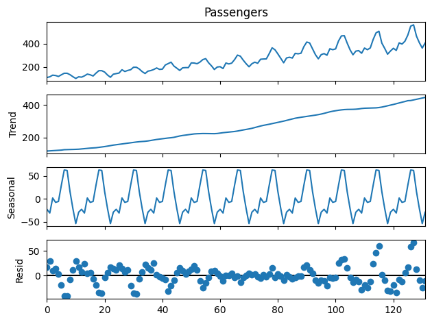
We can now clearly see both, a significantly increasing trend over the past 10 years as well as a recognizable seasonality pattern every year. Following those indications, we would now expect the model to predict some further increasing amount of passengers, following the seasonality peaks in the summer of the future year. But let’s try it out — time to apply some machine learning!

Model fitting with Facebook Prophet

To fit models in Prophet, it is important to have at least a ‘ds’ (datestamp) and ‘y’ (value to be forecasted) column. We should make sure that our columns are renamed the reflect the same.

df_train_prophet = df_data_train

# date variable needs to be named "ds" for prophet
df_train_prophet = df_train_prophet.rename(columns={"Month": "ds"})

# target variable needs to be named "y" for prophet
df_train_prophet = df_train_prophet.rename(columns={"Passengers": "y"})

Now the magic can begin. The process to fit the model is fairly straightforward. However, please have a look at the documentation to get an idea of the large amount of options and parameters we could adjust in this step. To keep things simple, we will fit a simple model without any further adjustments for now — but please keep in mind that real-world data is never perfect: you will definitely need parameter tuning in the future.

model_prophet  = Prophet()
model_prophet.fit(df_train_prophet)

That’s all we have to do to fit the model. Let’s make some predictions!

Making predictions

We have to make predictions on a table that has a ‘ds’ column with the dates you want predictions for. To set up this table, use the make_future_dataframe method, and it will automatically include historical dates. This way, you can see how well the model fits the past data and predicts the future. Since we handle monthly data, we will indicate the frequency with “freq=12″ and ask for a future horizon of 12 months (“periods=12”).

df_future = model_prophet.make_future_dataframe(periods=12, freq='MS')
display(df_future)

This new dataset then contains both, the training period as well as the additional 12 months we want to predict:

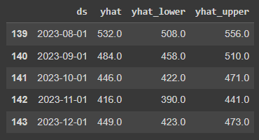
To make predictions, we simply call the predict method from Prophet and provide the future dataset. The prediction output will contain a large dataset with many different columns, but we will focus only on the predicted value yhat as well as the uncertainty intervals yhat_lower and yhat_upper.

forecast_prophet = model_prophet.predict(df_future)
forecast_prophet[['ds', 'yhat', 'yhat_lower', 'yhat_upper']].round().tail()

The table below gives us some idea about how the output is generated and stored. For August 2023, the model predicts a passenger amount of 532 people. The uncertainty interval (which is set by default to 80%) tells us in simple terms that we can expect most likely a passenger amount between 508 and 556 people in that month.

Finally, we want to visualize the output to better understand the predictions and the intervals.

Visualizing results

To plot the results, we can make use of Prophet’s built-in plotting tools. With the plot method, we can display the original time series data alongside the forecasted values.

import matplotlib.pyplot as plt

# plot the time series 
forecast_plot = model_prophet.plot(forecast_prophet)

# add a vertical line at the end of the training period
axes = forecast_plot.gca()
last_training_date = forecast_prophet['ds'].iloc[-12]
axes.axvline(x=last_training_date, color='red', linestyle='--', label='Training End')

# plot true test data for the period after the red line
df_data_test['Month'] = pd.to_datetime(df_data_test['Month'])
plt.plot(df_data_test['Month'], df_data_test['Passengers'],'ro', markersize=3, label='True Test Data')

# show the legend to distinguish between the lines
plt.legend()

Besides the general time series plot, we also added a dotted line to indicate the end of the training period and hence the start of the prediction period. Further, we made use of the true test dataset that we had prepared in the beginning.

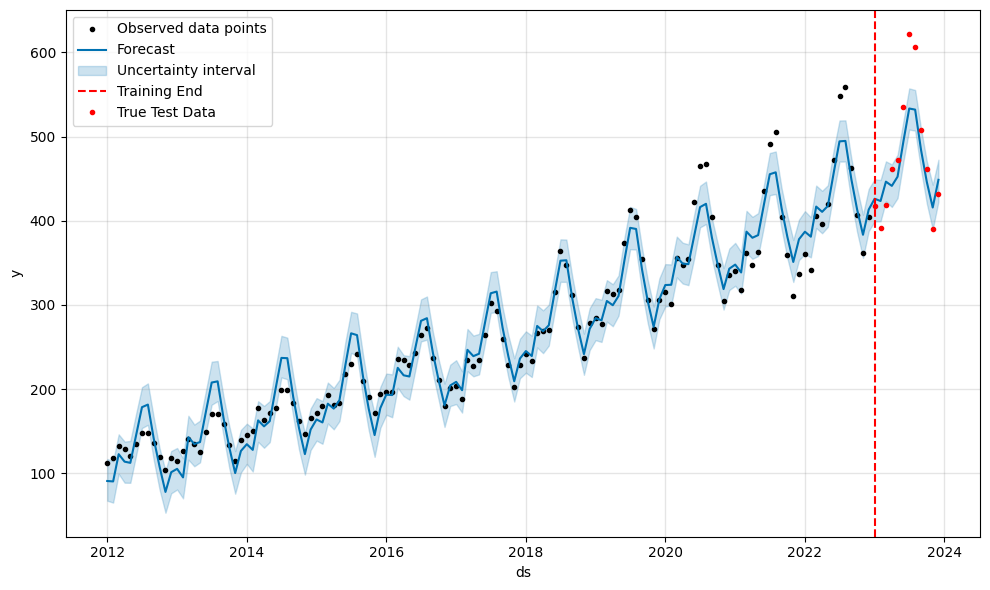
It can be seen that our model isn’t too bad. Most of the true passenger values are actually within the predicted uncertainty intervals. However, the summer months seem to be too pessimistic still, which is a pattern we can see in previous years already. This is a good moment to start exploring the parameters and features we could use with Prophet.

In our example, the seasonality is not a constant additive factor but it grows with the trend over time. Hence, we might consider changing the seasonality_mode from “additive” to “multiplicative” during the model fit. [4]

Our tutorial will conclude here to give some time to explore the large number of possibilities that Prophet offers to us. To review the full code together, I consolidated the snippets in this Python file. Additionally, you could upload this notebook directly to Colab and run it yourself. Let me know how it worked out for you!

Conclusion

Prophet is a powerful tool for predicting future values in time series data, especially when your data has repeating patterns like monthly or yearly cycles. It’s user-friendly and can quickly provide accurate predictions for your specific data. However, it’s essential to be aware of its limitations. If your data doesn’t have a clear pattern or if there are significant changes that the model hasn’t seen before, Prophet may not perform optimally. Understanding these limitations is crucial for using the tool wisely.

The good news is that experimenting with Prophet on your datasets is highly recommended! Every dataset is unique, and tweaking settings and trying different approaches can help you discover what works best for your specific situation. So, dive in, explore, and see how Prophet can enhance your time series forecasting.

Jonas Dieckmann – Medium

I hope you find it useful. Let me know your thoughts! And feel free to connect on LinkedIn https://www.linkedin.com/in/jonas-dieckmann/ and/or to follow me here on medium.

See also some of my other articles:

• How To Use ChatGPT API for Direct Interaction From Colab or Databricks
• How to get started with TensorFlow using Keras API and Google Colab

References

[1] Shumway, Robert H.; Stoffer, David S. (2017): Time Series Analysis and Its Applications. Cham: Springer International Publishing.

[2] Brownlee, Jason (2017): Introduction to Time Series Forecasting With Python

[3] Rafferty, Greg (2021): Forecasting Time Series Data with Facebook Prophet

[4] https://facebook.github.io/prophet/docs/quick_start.html

---

Getting started predicting time series data with Facebook Prophet was originally published in Towards Data Science on Medium, where people are continuing the conversation by highlighting and responding to this story.

The Math Behind the Adam Optimizer

Why is Adam the most popular optimizer in Deep Learning? Let’s understand it by diving into its math, and recreating the algorithm

If you’ve clicked on this article, you’ve likely heard about Adam, a name that has gained notable recognition in many winning Kaggle competitions. It’s common to experiment with a few optimizers like SGD, Adagrad, Adam, or AdamW, but truly understanding their mechanics is a different story. By the end of this post, you’ll be among the select few who not only know about Adam optimization but also understand how to leverage its power effectively.

By the way, in my previous post I described the math behind Stochastic Gradient Descent, if you missed it, I recommend reading it.

Stochastic Gradient Descent: Math and Python Code

Index

· 1: Understanding the Basics
∘ 1.1: What is the Adam Optimizer?
∘ 1.2: The Mechanics of Adam

· 2. Adam’s Algorithm Explained
∘ 2.1 The Mathematics Behind Adam
∘ 2.2 The Role of Adaptive Learning Rates

· 3. Adam in Practice
∘ 3.1 Recreating the Algorithm from Scratch in Python
∘ 3.2 Adam in TensorFlow

· 4. Advantages and Challenges
∘ 4.1 Why Opt for Adam?
∘ 4.2 Addressing Adam’s Limitations

· Conclusion

· Bibliography

1: Understanding the Basics

1.1: What is the Adam Optimizer?

In machine learning, Adam (Adaptive Moment Estimation) stands out as a highly efficient optimization algorithm. It’s designed to adjust the learning rates of each parameter.

Imagine you’re navigating a complex terrain, like the one in the image above. In some areas, you need to take large strides, while in others, cautious steps are required. Adam optimization works similarly, it dynamically adjusts its step size, making it larger in simpler regions and smaller in more complex ones, ensuring a more effective and quicker path to the lowest point, which represents the least loss in machine learning.

1.2: The Mechanics of Adam

Adam tweaks the gradient descent method by considering the moving average of the first and second-order moments of the gradient. This allows it to adapt the learning rates for each parameter intelligently.

At its core, Adam is designed to adapt to the characteristics of the data. It does this by maintaining individual learning rates for each parameter in your model. These rates are adjusted as the training progresses, based on the data it encounters.

Think of it as if you’re driving a car over different terrains. In some places, you accelerate (when the path is clear and straight), and in others, you decelerate (when the path gets twisty or rough). Adam modifies its speed (the learning rate_ based on the road (the gradient’s nature) ahead.

Indeed, the algorithm can remember the previous actions (gradients), and the new actions are guided by the previous ones. Therefore, Adams keeps track of the gradients from previous steps, allowing it to make informed adjustments to the parameters. This memory isn’t just a simple average; it’s a sophisticated combination of recent and past gradient information, giving more weight to the recent.

Moreover, in areas where the gradient (the slope of the loss function) changes rapidly or unpredictably, Adam takes smaller, more cautious steps. This helps avoid overshooting the minimum. Instead, in areas where the gradient changes slowly or predictably, it takes larger steps. This adaptability is key to Adam’s efficiency, as it navigates the loss landscape more intelligently than algorithms with a fixed step size.

This adaptability makes Adam particularly useful in scenarios where the data or the function being optimized is complex or has noisy gradients.

2. Adam’s Algorithm Explained

2.1 The Mathematics Behind Adam

As you may have understood, the core of Adam’s algorithm lies in its computation of adaptive learning rates for each parameter.

1. Initialization
In the beginning, Adam initializes two vectors, m, and v, which are both of the same shape as the parameters θ of the model. The vector m is intended to store the moving average of the gradients, while v keeps track of the moving average of the squared gradients. These moving averages are key to Adam’s adaptive adjustments. A time step counter t is also initialized to zero. It keeps track of the number of iterations (or updates) that the algorithm has completed.

The initial values are typically set as follows:

• m0​=0 (Initial first-moment vector)
• v0​=0 (Initial second-moment vector)
• t=0 (Time step)

2. Compute Gradients
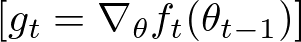
For each iteration t, Adam computes the gradient gt​. This gradient is the derivative of the objective function (which we are trying to minimize) concerning the current model parameters θt​.
Therefore, it represents the direction in which the function increases most rapidly.

Mathematically:

Where:

• gt​ represents the gradient at iteration t.
• ∇θ​ denotes the gradient for the parameters θ.
• ft​(θt−1​) is the objective function being optimized, evaluated at the parameter values from the previous iteration θt−1​.

3. Update m (first moment estimate)
Then, we update the first-moment vector m, which stores the moving average of the gradients.
This update is a combination of the previous value of m and the new gradient, weighted by parameters β1​ and 1−β1​, respectively.
This process can be likened to having a short-term memory of past gradients, emphasizing more recent observations. It provides a smoothed estimate of the gradient direction.

Mathematically:

Where:

• mt​ is the first-moment vector at time step t.
• β1​ is the exponential decay rate for the first moment estimates (commonly set to around 0.9).
• gt​ is the gradient at time step t.

4. Update v (second raw moment estimate)
Similarly, the second-moment vector v is updated. This vector gives an estimate of the variance (or unpredictability) of the gradients, therefore it stores the squared gradients that are accumulated.
Like the first moment, this is also a weighted combination, but of the past squared gradients and the current squared gradient.

Mathematically:

Where:

• vt​ is the second-moment vector at time step t.
• β2​ is the exponential decay rate for the second-moment estimates (commonly set to around 0.999).

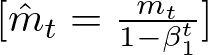
5. Correct the bias in the moments
Since m and v are initialized to 0, they are biased toward 0, which leads to a bias towards zero, especially during the initial time steps, particularly during the initial steps. Adam overcomes this bias by correcting the vector by the decay rate, which is b1 for m (first-moment decay rate), and b2 for v (second-moment decay rate).
This correction is important as it ensures that the moving averages are more representative, particularly in the early stages of training.

Mathematically:

Where:

• mt is the vector first-moment vector storing the moving average of the gradients at iteration t
• b1 is the decay rate of m at time t

Where​​:

• vt is the vector second-moment vector storing the variance of the gradients at iteration t
• b2 is the decay rate of vat time t

6. Update the parameters
The final step is the update of the model parameters. This step is where the actual optimization takes place, moving the parameters in the direction that minimizes the loss function. The update utilizes the adaptive learning rates calculated in the previous steps.

Mathematically:

Where:

• θt+1​ represents the parameters after the update.
• θt​ represents the current parameters before the update.
• α is the learning rate, a crucial hyperparameter that determines the size of the step taken toward the minimum of the loss function.
• m^t​ is the bias-corrected first moment (mean) estimate of the gradients.
• v^t​ is the bias-corrected second moment (uncentered variance) estimate of the gradients.
• ϵ (epsilon) is a small scalar (e.g., 10^-8) added to prevent division by zero and maintain numerical stability.

2.2 The Role of Adaptive Learning Rates

The key feature of Adam is its adaptive learning rates. Unlike traditional gradient descent, where a single learning rate is applied to all parameters, Adam adjusts the rate based on how frequently a parameter is updated.

Like in other optimization algorithms, the learning rate is a critical factor in how significantly the model parameters are adjusted. A higher learning rate could lead to faster convergence but risks overshooting the minimum, while a lower learning rate ensures more stable convergence but at the risk of getting stuck in local minima or taking too long to converge.

The unique aspect of Adam is that the update to each parameter is scaled individually. The amount by which each parameter is adjusted is influenced by both the first moment (capturing the momentum of the gradients) and the second moment (reflecting the variability of the gradients). This adaptive adjustment leads to more efficient and effective optimization, especially in complex models with many parameters.

The small constant ϵ is added to prevent any issues with division by zero, which is especially important when the second moment estimate v^t​ is very small. This addition is a standard practice in numerical algorithms to ensure stability.

3. Adam in Practice

3.1 Recreating the Algorithm from Scratch in Python

Now let’s move to the Python code, which really can make us understand how the algorithm works. In this example, I am recreating a simplified version of Adam, applied to Linear Regression. While, Adam is more commonly seen in the deep learning domain, building from scratch a Neural Network would require another post itself (follow me to stay updated, it’s coming…).
However, consider that you could replace the Linear Regression with other algorithms, as long as you adapt the code for it.

Let’s get started with creating the AdamOptimizer class first:

# Adam Optimizer (use the class from the previous response)
class AdamOptimizer:
    def __init__(self, learning_rate=0.001, beta1=0.9, beta2=0.999, epsilon=1e-8):
        """
        Constructor for the AdamOptimizer class.

        Parameters
        ----------
        learning_rate : float
            Learning rate for the optimizer.
        beta1 : float
            Exponential decay rate for the first moment estimates.
        beta2 : float
            Exponential decay rate for the second moment estimates.
        epsilon : float
            Small value to prevent division by zero.

        Returns
        -------
        None.
        """
        self.learning_rate = learning_rate
        self.beta1 = beta1
        self.beta2 = beta2
        self.epsilon = epsilon
        self.m = None
        self.v = None
        self.t = 0

    def initialize_moments(self, params):
        """
        Initializes the first and second moment estimates.

        Parameters
        ----------
        params : dict
            Dictionary containing the model parameters.
        
        Returns
        -------
        None.
        """
        self.m = {k: np.zeros_like(v) for k, v in params.items()}
        self.v = {k: np.zeros_like(v) for k, v in params.items()}

    def update_params(self, params, grads):
        """
        Updates the model parameters using the Adam optimizer.

        Parameters
        ----------
        params : dict
            Dictionary containing the model parameters.
        grads : dict
            Dictionary containing the gradients for each parameter.
        
        Returns
        -------
        updated_params : dict
            Dictionary containing the updated model parameters.
        """
        if self.m is None or self.v is None:
            self.initialize_moments(params)

        self.t += 1
        updated_params = {}

        for key in params.keys():
            self.m[key] = self.beta1 * self.m[key] + (1 - self.beta1) * grads[key]
            self.v[key] = self.beta2 * self.v[key] + (1 - self.beta2) * np.square(grads[key])

            m_corrected = self.m[key] / (1 - self.beta1 ** self.t)
            v_corrected = self.v[key] / (1 - self.beta2 ** self.t)

            updated_params[key] = params[key] - self.learning_rate * m_corrected / (np.sqrt(v_corrected) + self.epsilon)

        return updated_params

The code can be broken down into three parts:

Initialization of the class

def __init__(self, learning_rate=0.001, beta1=0.9, beta2=0.999, epsilon=1e-8):
        self.learning_rate = learning_rate
        self.beta1 = beta1
        self.beta2 = beta2
        self.epsilon = epsilon
        self.m = None
        self.v = None
        self.t = 0

Here, the class requests as inputs the learning rate, beta 1 (first-moment decay rate), beta 2 (second-moment decay rate), and epsilon.
Moreover, it temporarily sets the constants m, and v to None.

Initialization of the moment vectors

def initialize_moments(self, params):
        self.m = {k: np.zeros_like(v) for k, v in params.items()}
        self.v = {k: np.zeros_like(v) for k, v in params.items()}

In this step, we request an input “params”, a dictionary storing the model parameters. In the linear regression case, the model parameters are weight and bias, therefore we will expect two keys.

Then, we initialize two dictionaries: m, the first-moment vector, which will store the moving average of the gradients, and v, the second-moment vector, which will store the variance of the gradients.

Both of them will have several keys equal to the number of keys in the params dictionary (in our case two), and each key will have a value array with the same length as the values in the original key in params. In this case, the value array will store only 0 values, as we are initializing it.

Update the params dictionary

def update_params(self, params, grads):
        if self.m is None or self.v is None:
            self.initialize_moments(params)

        self.t += 1
        updated_params = {}

        for key in params.keys():
            self.m[key] = self.beta1 * self.m[key] + (1 - self.beta1) * grads[key]
            self.v[key] = self.beta2 * self.v[key] + (1 - self.beta2) * np.square(grads[key])

            m_corrected = self.m[key] / (1 - self.beta1 ** self.t)
            v_corrected = self.v[key] / (1 - self.beta2 ** self.t)

            updated_params[key] = params[key] - self.learning_rate * m_corrected / (np.sqrt(v_corrected) + self.epsilon)

        return updated_params

The last step is the core of the AdamOptimizer class, it will first start by initializing the first and second-moment vectors if they are not initialized.

Then, we update self.t, which is the time counter, which was originally set to 0, when we initialized the class. We, then create an empty updated_params dictionary, that will store the new model parameters after Adam optimization.

Lastly, we run the Adam optimization algorithm on the existing parameters, by iterating over every parameter with a for a loop. Since this is the main aspect of our operation let’s break it down:

self.m[key] = self.beta1 * self.m[key] + (1 - self.beta1) * grads[key]
self.v[key] = self.beta2 * self.v[key] + (1 - self.beta2) * np.square(grads[key])

These two lines of code update the first and second-moment vectors, using the formulas defined in subsection 2.1.

m_corrected = self.m[key] / (1 - self.beta1 ** self.t)
v_corrected = self.v[key] / (1 - self.beta2 ** self.t)

Here, we are updating the value in the two vectors by correcting them for the bias.

updated_params[key] = params[key] - self.learning_rate * m_corrected / (np.sqrt(v_corrected) + self.epsilon)

Lastly, we compute Adam optimization and store the new value in the updated_params dictionary.

Now, while this is technically the whole code we need for the Adam optimizer, this would be quite useless if we don’t have anything to optimize. Therefore, we will create a Linear Regression class to feed something to Adam.

# Linear Regression Model
class LinearRegression:
    def __init__(self, n_features):
        """
        Constructor for the LinearRegression class.

        Parameters
        ----------
        n_features : int
            Number of features in the input data.
        
        Returns
        -------
        None.
        """
        self.weights = np.random.randn(n_features)
        self.bias = np.random.randn()

    def predict(self, X):
        """
        Predicts the target variable given the input data.

        Parameters
        ----------
        X : numpy array
            Input data.

        Returns
        -------
        numpy array
            Predictions.
        """
        return np.dot(X, self.weights) + self.bias

This code is pretty self-explanatory. However, suppose you want to know more about Linear Regression and call yourself a Linear Regression master. In that case, I highly recommend you to read my article about it, where I recreate a more complex version of the one defined above.

Demystifying Linear Regression

Lastly, we define a wrapper class, which will combine both the Adam Optimizer class and the Linear Regression class:

class ModelTrainer:
    def __init__(self, model, optimizer, n_epochs):
        """
        Constructor for the ModelTrainer class.

        Parameters
        ----------
        model : object
            Model to be trained.
        optimizer : object
            Optimizer to be used for training.
        n_epochs : int
            Number of training epochs.

        Returns
        -------
        None.
        """
        self.model = model
        self.optimizer = optimizer
        self.n_epochs = n_epochs

    def compute_gradients(self, X, y):
        """
        Computes the gradients of the mean squared error loss function
        with respect to the model parameters.

        Parameters
        ----------
        X : numpy array
            Input data.
        y : numpy array
            Target variable.
        
        Returns
        -------
        dict
            Dictionary containing the gradients for each parameter.
        """
        predictions = self.model.predict(X)
        errors = predictions - y
        dW = 2 * np.dot(X.T, errors) / len(y)
        db = 2 * np.mean(errors)
        return {'weights': dW, 'bias': db}

    def train(self, X, y, verbose=False):
        """
        Runs the training loop, updating the model parameters and optionally printing the loss.

        Parameters
        ----------
        X : numpy array
            Input data.
        y : numpy array
            Target variable.
        
        Returns
        -------
        None.
        """
        for epoch in range(self.n_epochs):
            grads = self.compute_gradients(X, y)
            params = {'weights': self.model.weights, 'bias': self.model.bias}
            updated_params = self.optimizer.update_params(params, grads)

            self.model.weights = updated_params['weights']
            self.model.bias = updated_params['bias']

            # Optionally, print loss here to observe training
            loss = np.mean((self.model.predict(X) - y) ** 2)
            if epoch % 1000 == 0 and verbose:
                print(f"Epoch {epoch}, Loss: {loss}")

The main goal of the class is to iterate for several iterations given by the variable n_epochs optimizing the parameters of the linear regression by the Adam optimizer.

Compute the gradients

def compute_gradients(self, X, y):
        predictions = self.model.predict(X)
        errors = predictions - y
        dW = 2 * np.dot(X.T, errors) / len(y)
        db = 2 * np.mean(errors)
        return {'weights': dW, 'bias': db}

In this class, we finally compute the gradients. Indeed, in Subsection 2.1 that was the second step. Here it was not possible to calculate the gradients until we defined a model. Therefore, this function will vary based on the model you will feed to Adam. Since we are using Linear regression we only need to calculate the gradient of the weights and the bias.

Train

def train(self, X, y, verbose=False):
        for epoch in range(self.n_epochs):
            grads = self.compute_gradients(X, y)
            params = {'weights': self.model.weights, 'bias': self.model.bias}
            updated_params = self.optimizer.update_params(params, grads)

            self.model.weights = updated_params['weights']
            self.model.bias = updated_params['bias']

            loss = np.mean((self.model.predict(X) - y) ** 2)
            if epoch % 1000 == 0 and verbose:
                print(f"Epoch {epoch}, Loss: {loss}")

Finally, we create the train method. As we mentioned before, this class iterates n_epochs times. In each iteration, it computes the gradients of weights and bias resulting from Linear Regression, then feeds the gradients to the Adam optimizers, and sets the resulting weights and bias back to the model.

You can access the complete code with its implementation in a Jupyter Notebook here:

models-from-scratch-python/XGBoost/demo.ipynb at main · cristianleoo/models-from-scratch-python

3.2 Adam in TensorFlow

At this point, you will have a good understanding of the Adam optimizer. Now that you know how it works, you actually can discard the code above as you’ll likely use a more efficient implementation from Tensorflow or PyTorch with just a few lines of code.

In this case, we will use TensorFlow, and we will create a simple neural network with two layers and 64 nodes. Then, we will “compile” the model with Adam optimization. While compiling the optimizer is adjusting the weights of the network to minimize the loss.

import tensorflow as tf
import numpy as np

# Generate Sample Data
# For demonstration, we create synthetic data for a regression task
X = np.random.rand(100, 3)  # 100 samples, 3 features
y = X @ np.array([2.0, -1.0, 3.0]) + 1.5  # Linear relationship with some coefficients and bias

# Create the Neural Network
model = tf.keras.Sequential([
    tf.keras.layers.Dense(64, activation='relu', input_shape=(3,)),  # Input layer with 3 inputs
    tf.keras.layers.Dense(64, activation='relu'),  # Another dense layer
    tf.keras.layers.Dense(1)  # Output layer with 1 unit (for regression)
])

# Compile the Model with the Adam Optimizer
model.compile(optimizer=tf.keras.optimizers.Adam(learning_rate=0.001),
              loss='mean_squared_error')  # MSE is typical for regression

# Train the Model
model.fit(X, y, epochs=10)  # Train for 10 epochs as an example

4. Advantages and Challenges

4.1 Why Opt for Adam?

At this point, you know how the algorithm works, but you may still wondering when is Adam a good choice.

1. Dealing with Sparse Data
Adam is particularly effective when working with data that leads to sparse gradients. This situation is common in models with large embedding layers or when dealing with text data in natural language processing tasks.

2. Training Large-Scale Models
Adam is well-suited for training models with a large number of parameters, such as deep neural networks. Its adaptive learning rate helps navigate the complex optimization landscapes of such models efficiently. However, this is not always the case, as we can see when we applied Adam to Linear Regression.

3. Achieving Rapid Convergence
When we don’t have much time for the convergence to happen, Adam comes to help. This is thanks to its adaptive learning, which guarantees a faster convergence compared to its rival SGD.

4. For Online and Batch Training
It’s versatile enough to be used in both online learning scenarios (where the model is updated continuously as new data arrives) and batch learning.

4.2 Addressing Adam’s Limitations

While the Adam optimizer is versatile and effective in many scenarios, there are certain challenges and considerations to keep in mind.

1. Tuning Hyperparameters
While Adam is less sensitive to learning rate changes compared to other optimizers, choosing an appropriate initial learning rate is still crucial. A too-high learning rate may lead to instability, while too low a rate can slow down the training process.
The default values of β1​ and β2​ (typically 0.9 and 0.999, respectively) work well in most cases, but in some scenarios, adjusting them can yield better results.

2. Handling Noisy Data and Outliers
While Adam is generally robust to noisy data, extreme outliers or highly noisy datasets might impact its performance. Preprocessing data to remove or diminish the impact of outliers can be beneficial.

3. Choice of Loss Function
The efficiency of Adam can vary with different loss functions. Make sure that the loss function resonates with the problem you are solving, and experiment with a few of them to see which one works best.

4. Computational Considerations
Adam typically requires more memory than simple gradient descent algorithms because it maintains moving averages for each parameter. This should be considered when working with very large models or limited computational resources.

Conclusion

To effectively leverage Adam, it’s essential to understand both its strengths and limitations. Fine-tuning its parameters and being mindful of the nature of your data and problem can help in harnessing its full potential. Regular monitoring and validation are key to ensuring that the optimizer is performing optimally. Keep in mind these challenges, follow the best practices recommended in this article and you are ready to experiment with Adam.

Bibliography

1. Kingma, D. P., & Ba, J. (2014). Adam: A method for stochastic optimization. arXiv preprint arXiv:1412.6980. https://arxiv.org/abs/1412.6980
2. Ruder, S. (2016). An overview of gradient descent optimization algorithms. arXiv preprint arXiv:1609.04747. https://arxiv.org/abs/1609.04747
3. Goodfellow, I., Bengio, Y., & Courville, A. (2016). Deep Learning. MIT Press. http://www.deeplearningbook.org/

If you liked this article consider leaving a like, and follow me to be updated on my latest posts. My goal is to recreate all the most popular algorithms from scratch and make machine learning accessible to everyone.

---

The Math behind Adam Optimizer was originally published in Towards Data Science on Medium, where people are continuing the conversation by highlighting and responding to this story.