How to predict DAU using Duolingo’s growth model and control the prediction
1. Introduction
Doubtlessly, DAU, WAU, and MAU — daily, weekly, and monthly active users — are critical business metrics. An article “How Duolingo reignited user growth” by Jorge Mazal, former CPO of Duolingo, is #1 in the Growth section of Lenny’s Newsletter blog. In this article, Jorge paid special attention to the methodology Duolingo used to model the DAU metric (see another article “Meaningful metrics: how data sharpened the focus of product teams” by Erin Gustafson). This methodology has multiple strengths, but I’d like to focus on how one can use this approach for DAU forecasting.
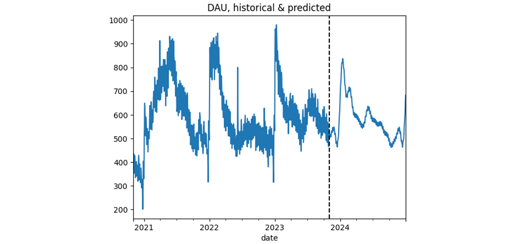
The new year is coming soon, so many companies are planning their budgets for the next year these days. Cost estimations often require DAU forecasts. In this article, I’ll show how you can get this prediction using Duolingo’s growth model. I’ll explain why this approach is better compared to standard time-series forecasting methods and how you can adjust the prediction according to your teams’ plans (e.g., marketing, activation, product teams).
The article text goes along with the code, and a simulated dataset is attached so the research is fully reproducible. The Jupyter notebook version is available here. In the end, I’ll share a DAU “calculator” designed in Google Spreadsheet format.
I’ll be narrating on behalf of the collective “we” as if we’re talking together.
2. Methodology
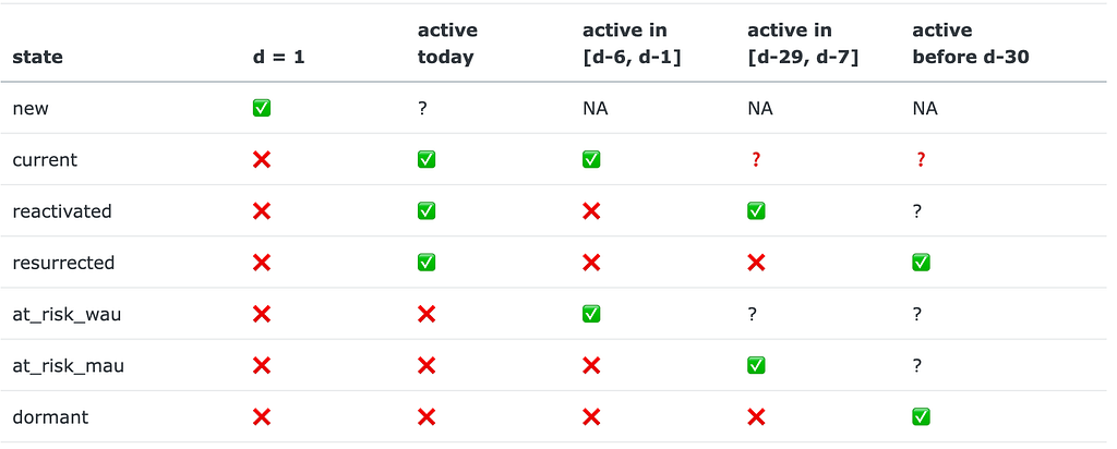
A quick recap on how the Duolingo’s growth model works. At day d (d = 1, 2, … ) of a user’s lifetime, the user can be in one of the following 7 (mutually-exclusive) states: new, current, reactivated, resurrected, at_risk_wau, at_risk_mau, dormant. The states are defined according to indicators of whether a user was active today, in the last 7 days, or in the last 30 days. The definition summary is given in the table below:
Having these states defined (as a set S), we can consider user behavior as a Markov chain. Here’s an example of a user’s trajectory: new→ current→ current→ at_risk_wau→…→ at_risk_mau→…→ dormant. Let M be a transition matrix associated with this Markov process: m_{i, j} = P(s_j | s_i) are the probabilities that a user moves to state s_j right after being at state s_i, where s_i, s_j ∈ S. Such a matrix is inferred from the historical data.
If we assume that user behavior is stationary (independent of time), the matrix M fully describes the states of all users in the future. Suppose that the vector u_0 of length 7 contains the counts of users in certain states on a given day, denoted as day 0. According to the Markov model, on the next day 1, we expect to have the following number of users states u_1:
Applying this formula recursively, we derive the number of users in certain states on any arbitrary day t > 0 in the future.
Besides the initial distribution u_0, we need to provide the number of new users that will appear in the product each day in the future. We’ll address this problem as a general time-series forecasting.
Now, having u_t calculated, we can determine DAU values on day t:
For each prediction day t = 1, …, T, calculate the expected number of new users #New_1, …, #New_T.
For each lifetime day of each user, assign one of the 7 states.
Calculate the transition matrix M from the historical data.
Calculate initial state counts u_0 corresponding to day t=0.
Recursively calculate u_{t+1} = M^T * u_t.
Calculate DAU, WAU, and MAU for each prediction day t = 1, …, T.
3. Implementation
This section is devoted to technical aspects of the implementation. If you’re interested in studying the model properties rather than code, you may skip this section and go to the Section 4.
3.1 Dataset
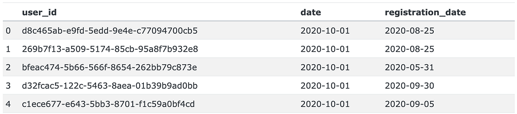
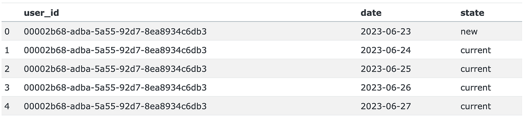
We use a simulated dataset based on historical data of a SaaS app. The data is stored in the dau_data.csv.gz file and contains three columns: user_id, date, and registration_date. Each record indicates a day when a user was active. The dataset includes activity indicators for 51480 users from 2020-11-01 to 2023-10-31. Additionally, data from October 2020 is included to calculate user states properly, as the at_risk_mau and dormant states require data from one month prior.
Suppose that today is 2023–10–31 and we want to predict the DAU metric for the next 2024 year. We define a couple of global constants PREDICTION_START and PREDICTION_END which encompass the prediction period.
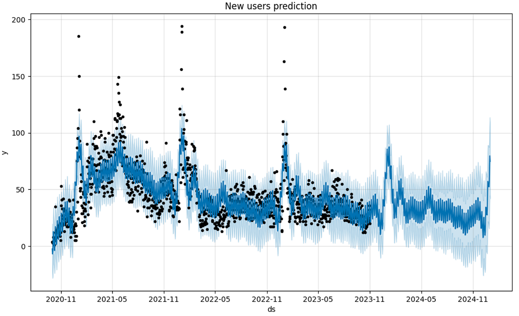
Let’s start from the new users prediction. We use the prophet library as one of the easiest ways to forecast time-series data. The new_users Series contains such data. We extract it from the original df dataset selecting the rows where the registration date is equal to the date.
prophet requires a time-series as a DataFrame containing two columns ds and y, so we reformat the new_users Series to the new_users_prophet DataFrame. Another thing we need to prepare is to create the future variable containing certain days for prediction: from prediction_start to prediction_end. This logic is implemented in the predict_new_users function. The plot below illustrates predictions for both past and future periods.
import logging import matplotlib.pyplot as plt from prophet import Prophet
def predict_new_users(prediction_start, prediction_end, new_users_train, show_plot=True): """ Forecasts a time-seires for new users
Parameters ---------- prediction_start : str Date in YYYY-MM-DD format. prediction_end : str Date in YYYY-MM-DD format. new_users_train : pandas.Series Historical data for the time-series preceding the prediction period. show_plot : boolean, default=True If True, a chart with the train and predicted time-series values is displayed. Returns ------- pandas.Series Series containing the predicted values. """ m = Prophet()
In practice, the most calculations are reasonable to execute as SQL queries to a database where the data is stored. Hereafter, we will simulate such querying using the duckdb library.
We want to assign one of the 7 states to each day of a user’s lifetime within the app. According to the definition, for each day, we need to consider at least the past 30 days. This is where SQL window functions come in. However, since the df data contains only records of active days, we need to explicitly extend them and include the days when a user was not active. In other words, instead of this list of records:
user_id    date          registration_date
1234567    2023-01-01    2023-01-01
1234567    2023-01-03    2023-01-01
query = f""" WITH full_range AS ( SELECT user_id, UNNEST(generate_series(greatest(registration_date, '{OBSERVATION_START}'), date '{DATASET_END}', INTERVAL 1 DAY))::date AS date FROM ( SELECT DISTINCT user_id, registration_date FROM df ) ), dau_full AS ( SELECT fr.user_id, fr.date, df.date IS NOT NULL AS is_active, registration_date FROM full_range AS fr LEFT JOIN df USING(user_id, date) ), states AS ( SELECT user_id, date, is_active, first_value(registration_date IGNORE NULLS) OVER (PARTITION BY user_id ORDER BY date) AS registration_date, SUM(is_active::int) OVER (PARTITION BY user_id ORDER BY date ROWS BETWEEN 6 PRECEDING and 1 PRECEDING) AS active_days_back_6d, SUM(is_active::int) OVER (PARTITION BY user_id ORDER BY date ROWS BETWEEN 29 PRECEDING and 1 PRECEDING) AS active_days_back_29d, CASE WHEN date = registration_date THEN 'new' WHEN is_active = TRUE AND active_days_back_6d BETWEEN 1 and 6 THEN 'current' WHEN is_active = TRUE AND active_days_back_6d = 0 AND IFNULL(active_days_back_29d, 0) > 0 THEN 'reactivated' WHEN is_active = TRUE AND active_days_back_6d = 0 AND IFNULL(active_days_back_29d, 0) = 0 THEN 'resurrected' WHEN is_active = FALSE AND active_days_back_6d > 0 THEN 'at_risk_wau' WHEN is_active = FALSE AND active_days_back_6d = 0 AND ifnull(active_days_back_29d, 0) > 0 THEN 'at_risk_mau' ELSE 'dormant' END AS state FROM dau_full ) SELECT user_id, date, state FROM states WHERE date BETWEEN '{DATASET_START}' AND '{DATASET_END}' ORDER BY user_id, date """ states = duckdb.sql(query).df()
The query results are kept in the states DataFrame:
3.4 Calculating the transition matrix
Having obtained these states, we can calculate state transition frequencies. In the Section 4.3 we’ll study how the prediction depends on a period in which transitions are considered, so it’s reasonable to pre-aggregate this data on daily basis. The resulting transitions DataFrame contains date, state_from, state_to, and cnt columns.
Now, we can calculate the transition matrix M. We implement the get_transition_matrix function, which accepts the transitions DataFrame and a pair of dates that encompass the transitions period to be considered.
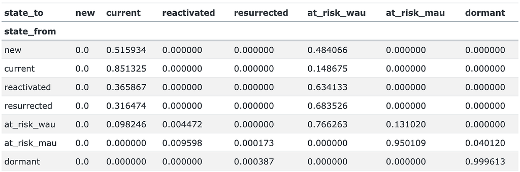
As a baseline, let’s calculate the transition matrix for the whole year from 2022-11-01 to 2023-10-31.
M = get_transition_matrix(transitions, '2022-11-01', '2023-10-31')
M
The sum of each row of any transition matrix equals 1 since it represents the probabilities of moving from one state to any other state.
3.5 Getting the initial state counts
An initial state is retrieved from the states DataFrame by the get_state0 function and the corresponding SQL query. The only argument of the function is the date for which we want to get the initial state. We assign the result to the state0 variable.
def get_state0(date): query = f""" SELECT state, count(*) AS cnt FROM states WHERE date = '{date}' GROUP BY state """
state
new               20
current          475
reactivated       15
resurrected       19
at_risk_wau      404
at_risk_mau     1024
dormant        49523
Name: cnt, dtype: int64
3.6 Predicting DAU
The predict_dau function below accepts all the previous variables required for the DAU prediction and makes this prediction for a date range defined by the start_date and end_date arguments.
def predict_dau(M, state0, start_date, end_date, new_users): """ Predicts DAU over a given date range.
Parameters ---------- M : pandas.DataFrame Transition matrix representing user state changes. state0 : pandas.Series counts of initial state of users. start_date : str Start date of the prediction period in 'YYYY-MM-DD' format. end_date : str End date of the prediction period in 'YYYY-MM-DD' format. new_users : int or pandas.Series The expected amount of new users for each day between `start_date` and `end_date`. If a Series, it should have dates as the index. If an int, the same number is used for each day.
Returns ------- pandas.DataFrame DataFrame containing the predicted DAU, WAU, and MAU for each day in the date range, with columns for different user states and tot. """
dates = pd.date_range(start_date, end_date) dates.name = 'date' dau_pred = [] new_dau = state0.copy() for date in dates: new_dau = (M.transpose() @ new_dau).astype(int) if isinstance(new_users, int): new_users_today = new_users else: new_users_today = new_users.astype(int).loc[date] new_dau.loc['new'] = new_users_today dau_pred.append(new_dau.tolist())
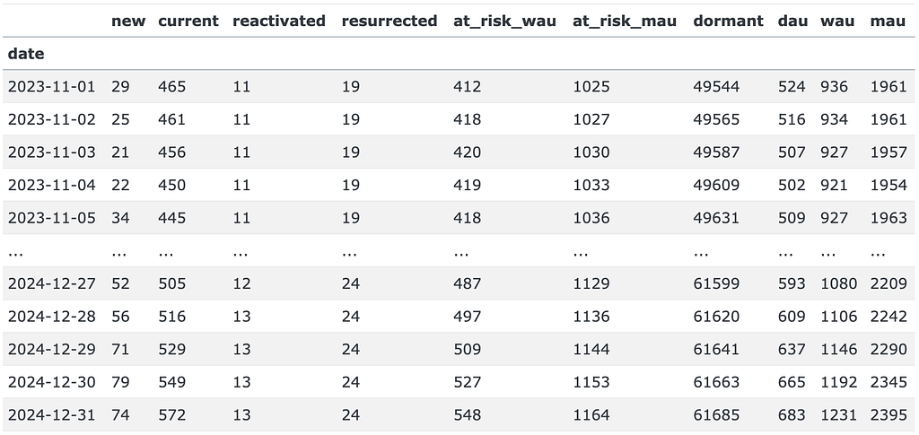
This is how the DAU prediction dau_pred looks like for the PREDICTION_START – PREDICTION_END period. Besides the expected dau, wau, and mau columns, the output contains the number of users in each state for each prediction date.
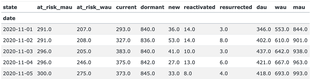
Finally, we calculate the ground-truth values of DAU, WAU, and MAU (along with the user state counts), keep them in the dau_true DataFrame, and plot the predicted and true values altogether.
query = f""" SELECT date, state, COUNT(*) AS cnt FROM states GROUP BY date, state ORDER BY date, state; """
We’ve obtained the prediction but so far it’s not clear whether it’s fair or not. In the next section, we’ll evaluate the model.
4. Model evaluation
4.1 Baseline model
First of all, let’s check whether we really need to build a complex model to predict DAU. Wouldn’t it be better to predict DAU as a general time-series using the mentioned prophet library? The function predict_dau_prophet below implements this. We try to use some tweaks available in the library in order to make the prediction more accurate. In particular:
we use logistic model instead of linear to avoid negative values;
we add explicitly monthly and yearly seasonality;
we remove the outliers;
we explicitly define a peak period in January and February as “holidays”.
def predict_dau_prophet(prediction_start, prediction_end, dau_true, show_plot=True): # assigning peak days for the new year holidays = pd.DataFrame({ 'holiday': 'january_spike', 'ds': pd.date_range('2022-01-01', '2022-01-31', freq='D').tolist() + pd.date_range('2023-01-01', '2023-01-31', freq='D').tolist(), 'lower_window': 0, 'upper_window': 40 })
m = Prophet(growth='logistic', holidays=holidays) m.add_seasonality(name='monthly', period=30.5, fourier_order=3) m.add_seasonality(name='yearly', period=365, fourier_order=3)
# converting the predictions to an appropriate format pred = pred .assign(yhat=lambda _df: _df['yhat'].astype(int)) .rename(columns={'ds': 'date', 'yhat': 'count'}) .set_index('date') .clip(lower=0) ['count'] .loc[lambda s: (s.index >= prediction_start) & (s.index <= prediction_end)]
return pred
The fact that the code turns out to be quite sophisticated indicates that one can’t simply apply prophet to the DAU time-series.
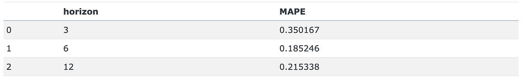
Hereafter we test a prediction for multiple predicting horizons: 3, 6, and 12 months. As a result, we get 3 test sets:
3-months horizon: 2023-08-01 – 2023-10-31,
6-months horizon: 2023-05-01 – 2023-10-31,
1-year horizon: 2022-11-01 – 2023-10-31.
For each test set we calculate the MAPE loss function.
from sklearn.metrics import mean_absolute_percentage_error
The MAPE error turns out to be high: 18% — 35%. The fact that the shortest horizon has the highest error means that the model is tuned for the long-term predictions. This is another inconvenience of such an approach: we have to tune the model for each prediction horizon. Anyway, this is our baseline. In the next section we’ll compare it with more advanced models.
4.2 General evaluation
In this section we evaluate the model implemented in the Section 3.6. So far we set the transition period as 1 year before the prediction start. We’ll study how the prediction depends on the transition period in the Section 4.3. As for the new users, we run the model using two options: the real values and the predicted ones. Similarly, we fix the same 3 prediction horizons and test the model on them.
The make_predicion helper function below implements the described options. It accepts prediction_start, prediction_end arguments defining the prediction period for a given horizon, new_users_mode which can be either true or predict, and transition_period. The options of the latter argument will be explained further.
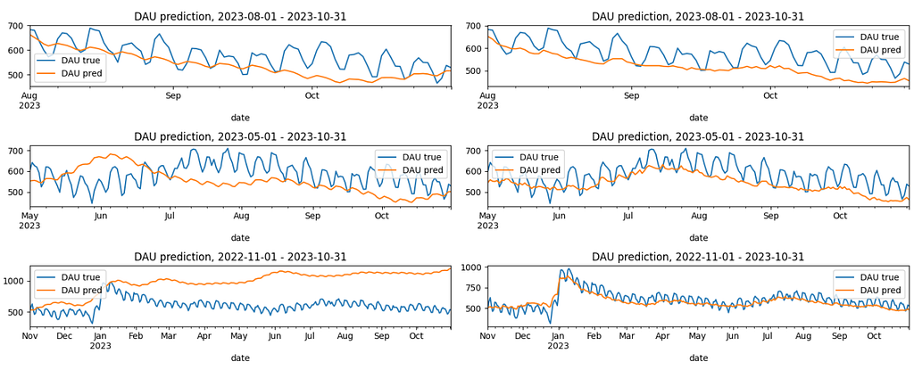
In total, we have 6 prediction scenarios: 2 options for new users and 3 prediction horizons. The diagram below illustrates the results. The charts on the left relate to the new_users_mode = ‘predict’ option, while the right ones relate to the new_users_mode = ‘true’ option.
In general, the model demonstrates much better results than the baseline. Indeed, the baseline is based on the historical DAU data only, while the model uses the user states information.
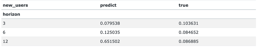
However, for the 1-year horizon and new_users_mode=’predict’ the MAPE error is huge: 65%. This is 3 times higher than the corresponding baseline error (21%). On the other hand, new_users_mode=’true’ option gives a much better result: 8%. It means that the new users prediction has a huge impact on the model, especially for long-term predictions. For the shorter periods the difference is less dramatic. The major reason for such a difference is that 1-year period includes Christmas with its extreme values. As a result, i) it’s hard to predict such high new user values, ii) the period heavily impacts user behavior, the transition matrix and, consequently, DAU values. Hence, we strongly recommend to implement the new user prediction carefully. The baseline model was specially tuned for this Christmas period, so it’s not surprising that it outperforms the Markov model.
When the new users prediction is accurate, the model captures trends well. It means that using last 365 days for the transition matrix calculation is a reasonable choice.
Interestingly, the true new users data provides worse results for the 3-months prediction. This is nothing but a coincidence. The wrong new users prediction in October 2023 reversed the predicted DAU trend and made MAPE a bit lower.
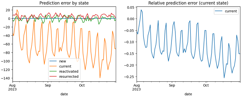
Now, let’s decompose the prediction error and see which states contribure the most. By error we mean here dau_pred – dau_true values, by relative error – ( dau_pred – dau_true) / dau_true – see left and right diagrams below correspondingly. In order to focus on this aspect, we’ll narrow the configuration to the 3-months prediction horizon and the new_users_mode=’true’ option.
From the left chart we notice that the error is basically contributed by the current state. It’s not surprising since this state contributes to DAU the most. The error for the reactivated, and resurrected states is quite low. Another interesting thing is that this error is mostly negative for the current state and mostly positive for the resurrected state. The former might be explained by the fact that the new users who appeared in the prediction period are more engaged that the users from the past. The latter indicates that the resurrected users in reality contribute to DAU less than the transition matrix expects, so the dormant→ resurrected conversion rate is overestimated.
As for the relative error, it makes sense to analyze it for the current state only. This is because the daily amount of the reactivated and resurrected states are low so the relative error is high and noisy. The relative error for the current state varies between -25% and 4% which is quite high. And since we’ve fixed the new users prediction, this error is explained by the transition matrix inaccuracy only. In particular, the current→ current conversion rate is roughly 0.8 which is high and, as a result, it contributes to the error a lot. So if we want to improve the prediction we need to consider tuning this conversion rate foremost.
4.3 Transitions period impact
In the previous section we kept the transitions period fixed: 1 year before a prediction start. Now we’re going to study how long this period should be to get more accurate prediction. We consider the same prediction horizons of 3, 6, and 12 months. In order to mitigate the noise from the new users prediction, we use the real values of the new users amount: new_users_mode=’true’.
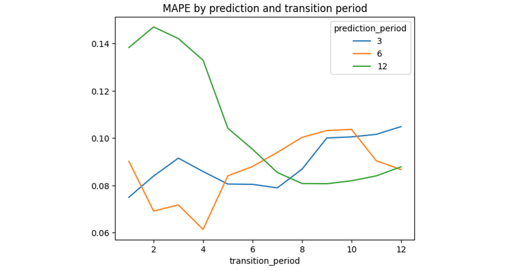
Here comes varying of the transition_period argument. Its values are masked with the last_<N>d pattern where N stands for the number of days in a transitions period. For each prediction horizon we calculate 12 different transition periods of 1, 2, …, 12 months. Then we calculate the MAPE error for each of the options and plot the results.
result = []

for prediction_offset in prediction_horizon:
    prediction_start = pd.to_datetime(prediction_end) - pd.DateOffset(months=prediction_offset - 1)
    prediction_start = prediction_start.replace(day=1)

    for transition_offset in range(1, 13):
        dau_pred = make_prediction(
            prediction_start, prediction_end, new_users_mode='true',
            transition_period=f'last_{transition_offset*30}d'
        )
        mape = prediction_details(dau_true, dau_pred, show_plot=False)
        result.append([prediction_offset, transition_offset, mape])
result = pd.DataFrame(result, columns=['prediction_period', 'transition_period', 'mape'])

result.pivot(index='transition_period', columns='prediction_period', values='mape')
    .plot(title='MAPE by prediction and transition period');
It turns out that the optimal transitions period depends on the prediction horizon. Shorter horizons require shorter transitions periods: the minimal MAPE error is achieved at 1, 4, and 8 transition periods for the 3, 6, and 12 months correspondingly. Apparently, this is because the longer horizons contain some seasonal effects that could be captured only by the longer transitions periods. Also, it seems that for the longer prediction horizons the MAPE curve is U-shaped meaning that too long and too short transitions periods are both not good for the prediction. We’ll develop this idea in the next section.
4.4 Obsolence and seasonality
Nevertheless, fixing a single transition matrix for predicting the whole year ahead doesn’t seem to be a good idea: such a model would be too rigid. Usually, user behavior varies depending on a season. For example, users who appear after Christmas might have some shifts in behavior. Another typical situation is when users change their behavior in summer. In this section, we’ll try to take into account these seasonal effects.
So we want to predict DAU for 1 year ahead starting from November 2022. Instead of using a single transition matrix M_base which is calculated for the last 8 months before the prediction start, according to the previous subsection results (and labeled as the last_240d option below), we’ll consider a mixture of this matrix and a seasonal one M_seasonal. The latter is calculated on monthly basis lagging 1 year behind. For example, to predict DAU for November 2022 we define M_seasonal as the transition matrix for November 2021. Then we shift the prediction horizon to December 2022 and calculate M_seasonal for December 2021, etc.
In order to mix M_base and M_seasonal we define the following two options.
seasonal_0.3: M = 0.3 * M_seasonal + 0.7 * M_base. 0.3 is a weight that was chosen as a local minimum after some experiments.
smoothing: M = i/(N-1) * M_seasonal + (1 – i/(N – 1)) * M_base where N is the number of months within the predicting period, i = 0, …, N – 1 – the month index. The idea of this configuration is to gradually switch from the most recent transition matrix M_base to seasonal ones as the prediction month moves forward from the prediction start.
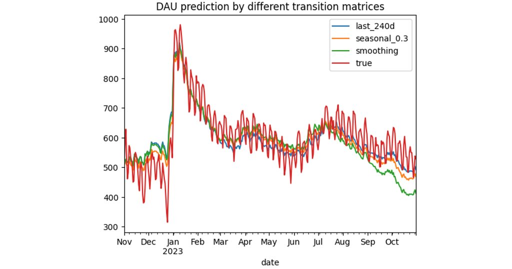
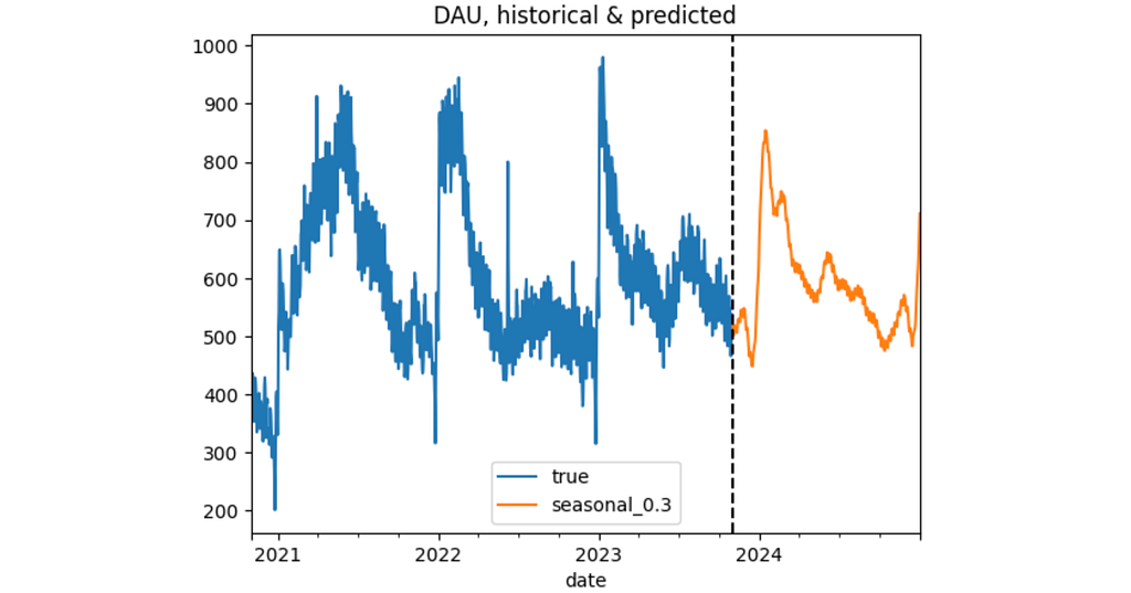
result = pd.DataFrame()
for transition_period in ['last_240d', 'seasonal_0.3', 'smoothing']:
    result[transition_period] = make_prediction(
        '2022-11-01', '2023-10-31',
        'true',
        transition_period
    )['dau']
result['true'] = dau_true['dau']
result['true'] = result['true'].astype(int)
result.plot(title='DAU prediction by different transition matrices');
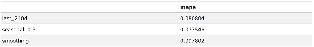
mape = pd.DataFrame()
for col in result.columns:
    if col != 'true':
        mape.loc[col, 'mape'] = mean_absolute_percentage_error(result['true'], result[col])
mape
According to the MAPE errors, seasonal_0.3 configuration provides the best results. Interestingly, smoothing approach has appeared to be even worse than the last_240d. From the diagram above we see that all three models start to underestimate the DAU values in July 2023, especially the smoothing model. It seems that the new users who started appearing in July 2023 are more engaged than the users from 2022. Probably, the app was improved sufficiently or the marketing team did a great job. As a result, the smoothing model that much relies on the outdated transitions data from July 2022 – October 2022 fails more than the other models.
4.5 Final solution
To sum things up, let’s make a final prediction for the 2024 year. We use the seasonal_0.3 configuration and the predicted values for new users.
In the Section 4 we studied the model performance from the prediction accuracy perspective. Now let’s discuss the model from the practical point of view.
Besides poor accuracy, predicting DAU as a time-series (see the Section 4.1) makes this approach very stiff. Essentially, it makes a prediction in such a manner so it would fit historical data best. In practice, when making plans for a next year we usually have some certain expectations about the future. For example,
the marketing team is going to launch some new more effective campaings,
the activation team is planning to improve the onboarding process,
the product team will release some new features that would engage and retain users more.
Our model can take into account such expectations. For the examples above we can adjust the new users prediction, the new→ current and the current→ current conversion rates respectively. As a result, we can get a prediction that doesn’t match with the historical data but nevertheless would be more realistic. This model’s property is not just flexible – it’s interpretable. You can easily discuss all these adjustments with the stakeholders, and they can understand how the prediction works.
Another advantage of the model is that it doesn’t require predicting whether a certain user will be active on a certain day. Sometimes binary classifiers are used for this purpose. The downside of this approach is that we need to apply such a classifier to each user including all the dormant users and each day from a prediction horizon. This is a tremedous computational cost. In contrast, the Markov model requires only the initial amount of states ( state0). Moreover, such classiffiers are often black-box models: they are poorly interpretable and hard to adjust.
The Markov model also has some limitations. As we already have seen, it’s sensitive to the new users prediction. It’s easy to totally ruin the prediction by a wrong new users amount. Another problem is that the Markov model is memoryless meaning that it doesn’t take into account the user’s history. For example, it doesn’t distinguish whether a current user is a newbie, experienced, or reactivated/ resurrected one. The retention rate of these user types should be certainly different. Also, as we discussed earlier, the user behavior might be of different nature depending on the season, marketing sources, countries, etc. So far our model is not able to capture these differences. However, this might be a subject for further research: we could extend the model by fitting more transition matrices for different user segments.
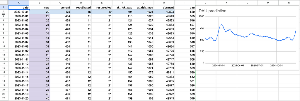
Finally, as we promised in the introduction, we provide a DAU spreadsheet calculator. In the Prediction sheet you’ll need to fill the initial states distribution row (marked with blue) and the new users prediction column (marked with purple). In the Conversions sheet you can adjust the transition matrix values. Remember that the sum of each row of the matrix should be equal to 1.
That’s all for now. I hope that this article was useful for you. In case of any questions or suggestions, feel free to ask in the comments below or contact me directly on LinkedIn.
All the images in the post are generated by the author.
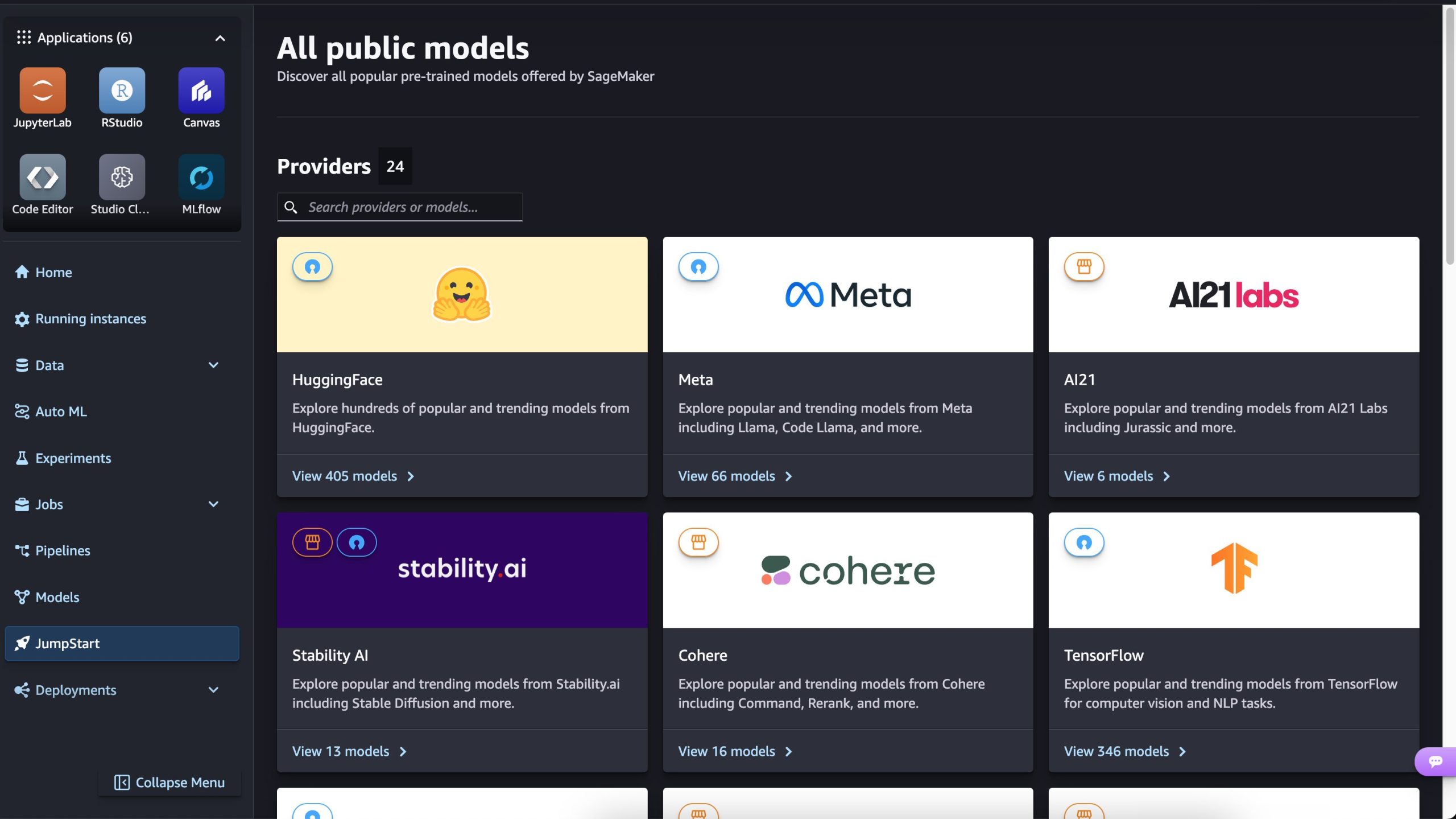
Today, we are excited to announce that Mistral-NeMo-Base-2407 and Mistral-NeMo-Instruct-2407 large language models from Mistral AI that excel at text generation, are available for customers through Amazon SageMaker JumpStart. In this post, we walk through how to discover, deploy and use the Mistral-NeMo-Instruct-2407 and Mistral-NeMo-Base-2407 models for a variety of real-world use cases.
Large Language models are comprised of billions of parameters (weights). For each word it generates, the model has to perform computationally expensive calculations across all of these parameters.
Large Language models accept a sentence, or sequence of tokens, and generate a probability distribution of the next most likely token.
Thus, typically decoding n tokens (or generating n words from the model) requires running the model n number of times. At each iteration, the new token is appended to the input sentence and passed to the model again. This can be costly.
Additionally, decoding strategy can influence the quality of the generated words. Generating tokens in a simple way, by just taking the token with the highest probability in the output distribution, can result in repetitive text. Random sampling from the distribution can result in unintended drift.
Thus, a solid decoding strategy is required to ensure both:
High Quality Outputs
Fast Inference Time
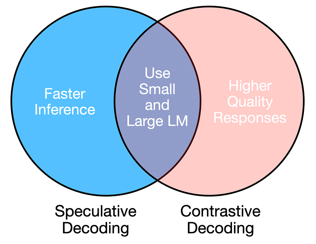
Both requirements can be addressed by using a combination of a large and small language model, as long as the amateur and expert models are similar (e.g., same architecture but different sizes).
Target/Large Model: Main LM with larger number of parameters (e.g. OPT-13B)
Amateur/Small Model: Smaller version of Main LM with fewer parameters (e.g. OPT-125M)
Speculative and contrastive decoding leverage large and small LLMs to achieve reliable and efficient text generation.
Contrastive Decoding for High Quality Inference
Contrastive Decoding is a strategy that exploits the fact that that failures in large LLMs (such as repetition, incoherence) are even more pronounced in small LLMs. Thus, this strategy optimizes for the tokens with the highest probability difference between the small and large model.
For a single prediction, contrastive decoding generates two probability distributions:
q = logit probabilities for amateur model
p = logit probabilities for expert model
The next token is chosen based on the following criteria:
Discard all tokens that do not have sufficiently high probability under the expert model (discard p(x) < alpha * max(p))
From the remaining tokens, select the one the with the largest difference between large model and small model log probabilities, max(p(x) – q(x)).
Implementing Contrastive Decoding
from transformers import AutoTokenizer, AutoModelForCausalLM import torch
# Set an alpha threshold to eliminate less confident tokens in expert alpha = 0.1 candidate_exp_prob = torch.max(expert_logits)
# Mask tokens below threshold for expert model V_head = expert_logits < alpha * candidate_exp_prob
# Select the next token from the log-probabilities difference, ignoring masked values token = torch.argmax(log_probs_diff.masked_fill(V_head, -torch.inf)).unsqueeze(0)
# Append token and accumulate generated text input_ids = torch.cat([input_ids, token.unsqueeze(1)], dim=-1)
Speculative decoding is based on the principle that the smaller model must sample from the same distribution as the larger model. Thus, this strategy aims to accept as many predictions from the smaller model as possible, provided they align with the distribution of the larger model.
The smaller model generates n tokens in sequence, as possible guesses. However, all n sequences are fed into the larger expert model as a single batch, which is faster than sequential generation.
This results in a cache for each model, with n probability distributions in each cache.
q = logit probabilities for amateur model
p = logit probabilities for expert model
Next, the sampled tokens from the amateur model are accepted or rejected based on the following conditions:
If probability of the token is higher in expert distribution (p) than amateur distribution (q), or p(x) > q(x), accept token
If probability of token is lower in expert distribution (p) than amateur distribution (q), or p(x) < q(x), reject token with probability 1 – p(x) / q(x)
If a token is rejected, the next token is sampled from the expert distribution or adjusted distribution. Additionally, the amateur and expert model reset the cache and re-generate n guesses and probability distributions p and q.
Here, the blue signifies accepted tokens, and red/green signify tokens rejected and then sampled from the expert or adjusted distribution.
Implementing Speculative Decoding
from transformers import AutoTokenizer, AutoModelForCausalLM import torch
# Sample a token from the adjusted expert distribution normalized_result = clipped_diff / torch.sum(clipped_diff, dim=0, keepdim=True) next_token = sample_from_distribution(normalized_result) input_ids = torch.cat([input_ids, next_token.unsqueeze(1)], dim=-1) else: # Sample directly from the expert logits for the last accepted token next_token = sample_from_distribution(expert_logits[-1]) input_ids = torch.cat([input_ids, next_token.unsqueeze(1)], dim=-1)
return tokenizer.batch_decode(input_ids)
# Example usage prompt = "Large Language models are" generated_text = speculative_decoding(prompt, n_tokens=3, max_length=25) print(generated_text)
Evaluation
We can evaluate both decoding approaches by comparing them to a naive decoding method, where we randomly pick the next token from the probability distribution.
def sequential_sampling(prompt, max_length=50): """ Perform sequential sampling with the given model. """ # Tokenize the input prompt input_ids = tokenizer(prompt, return_tensors="pt").input_ids
with torch.no_grad(): while input_ids.shape[1] < max_length: # Sample from the model output logits for the last token outputs = expert_lm(input_ids, return_dict=True) logits = outputs.logits[:, -1, :]
To evaluate contrastive decoding, we can use the following metrics for lexical richness.
n-gram Entropy: Measures the unpredictability or diversity of n-grams in the generated text. High entropy indicates more diverse text, while low entropy suggests repetition or predictability.
distinct-n: Measures the proportion of unique n-grams in the generated text. Higher distinct-n values indicate more lexical diversity.
from collections import Counter import math
def ngram_entropy(text, n): """ Compute n-gram entropy for a given text. """ # Tokenize the text tokens = text.split() if len(tokens) < n: return 0.0 # Not enough tokens to form n-grams
# Create n-grams ngrams = [tuple(tokens[i:i + n]) for i in range(len(tokens) - n + 1)]
# Compute entropy entropy = -sum((count / total_ngrams) * math.log2(count / total_ngrams) for count in ngram_counts.values()) return entropy
def distinct_n(text, n): """ Compute distinct-n metric for a given text. """ # Tokenize the text tokens = text.split() if len(tokens) < n: return 0.0 # Not enough tokens to form n-grams
# Create n-grams ngrams = [tuple(tokens[i:i + n]) for i in range(len(tokens) - n + 1)]
# Count unique and total n-grams unique_ngrams = set(ngrams) total_ngrams = len(ngrams)
return len(unique_ngrams) / total_ngrams if total_ngrams > 0 else 0.0
prompts = [ "Large Language models are", "Barack Obama was", "Decoding strategy is important because", "A good recipe for Halloween is", "Stanford is known for" ]
for n in range(1, 4): contrastive_entropy_totals[n - 1] += ngram_entropy(contrastive_generated_text, n)
for n in range(1, 3): contrastive_distinct_totals[n - 1] += distinct_n(contrastive_generated_text, n)
# Compute averages naive_entropy_averages = [total / len(prompts) for total in naive_entropy_totals] naive_distinct_averages = [total / len(prompts) for total in naive_distinct_totals] contrastive_entropy_averages = [total / len(prompts) for total in contrastive_entropy_totals] contrastive_distinct_averages = [total / len(prompts) for total in contrastive_distinct_totals]
# Display results print("Naive Sampling:") for n in range(1, 4): print(f"Average Entropy (n={n}): {naive_entropy_averages[n - 1]}") for n in range(1, 3): print(f"Average Distinct-{n}: {naive_distinct_averages[n - 1]}")
print("nContrastive Decoding:") for n in range(1, 4): print(f"Average Entropy (n={n}): {contrastive_entropy_averages[n - 1]}") for n in range(1, 3): print(f"Average Distinct-{n}: {contrastive_distinct_averages[n - 1]}")
The following results show us that contrastive decoding outperforms naive sampling for these metrics.
Naive Sampling: Average Entropy (n=1): 4.990499826537679 Average Entropy (n=2): 5.174765791328267 Average Entropy (n=3): 5.14373124004409 Average Distinct-1: 0.8949694135740648 Average Distinct-2: 0.9951219512195122
Contrastive Decoding: Average Entropy (n=1): 5.182773920916605 Average Entropy (n=2): 5.3495681172235665 Average Entropy (n=3): 5.313720275712986 Average Distinct-1: 0.9028425204970866 Average Distinct-2: 1.0
To evaluate speculative decoding, we can look at the average runtime for a set of prompts for different n values.
prompts = [ "Large Language models are", "Barack Obama was", "Decoding strategy is important because", "A good recipe for Halloween is", "Stanford is known for" ]
# Loop through n_tokens values for n in n_tokens: avg_time_naive, avg_time_speculative = 0, 0
for prompt in prompts: start_time = time.time() _ = sequential_sampling(prompt, max_length=25) avg_time_naive += (time.time() - start_time)
# Labels and title plt.xlabel('n_tokens', fontsize=12) plt.ylabel('Average Time (s)', fontsize=12) plt.title('Speculative Decoding Runtime vs n_tokens', fontsize=14) plt.legend() plt.grid(axis='y', linestyle='--', alpha=0.7)
# Show the plot plt.show() plt.savefig("plot.png")
We can see that the average runtime for the naive decoding is much higher than for speculative decoding across n values.
Combining large and small language models for decoding strikes a balance between quality and efficiency. While these approaches introduce additional complexity in system design and resource management, their benefits apply to conversational AI, real-time translation, and content creation.
These approaches require careful consideration of deployment constraints. For instance, the additional memory and compute demands of running dual models may limit feasibility on edge devices, though this can be mitigated through techniques like model quantization.
Unless otherwise noted, all images are by the author.
Anyone who has tried teaching a dog new tricks knows the basics of reinforcement learning. We can modify the dog’s behavior by repeatedly offering rewards for obedience and punishments for misbehavior. In reinforcement learning (RL), the dog would be an agent, exploring its environment and receiving rewards or penalties based on the available actions. This very simple concept has been formalized mathematically and extended to advance the fields of self-driving and self-driving/autonomous labs.
As a New Yorker, who finds herself riddled with anxiety driving, the benefits of having a stoic robot chauffeur are obvious. The benefits of an autonomous lab only became apparent when I considered the immense power of the new wave of generative AI biology tools. We can generate a huge volume of high-quality hypotheses and are now bottlenecked by experimental validation.
If we can utilize reinforcement learning (RL) to teach a car to drive itself, can we also use it to churn through experimental validations of AI-generated ideas? This article will continue our series, Understanding AI Applications in Bio for ML Engineers, by learning how reinforcement learning is applied in self-driving cars and autonomous labs (for example, AlphaFlow).
Self-Driving Cars
The most general way to think about RL is that it’s a learning method by doing. The agent interacts with its environment, learns what actions produce the highest rewards, and avoids penalties through trial and error. If learning through trial and error going 65mph in a 2-ton metal box sounds a bit terrifying, and like something that a regulator would not approve of, you’d be correct. Most RL driving has been done in simulation environments, and current self-driving technology still focuses on supervised learning techniques. But Alex Kendall proved that a car could teach itself to drive with a couple of cheap cameras, a massive neural network, and twenty minutes. So how did he do it?
More mainstream self driving approaches use specialized modules for each of subproblem: vehicle management, perception, mapping, decision making, etc. But Kendalls’s team used a deep reinforcement learning approach, which is an end-to-end learning approach. This means, instead of breaking the problem into many subproblems and training algorithms for each one, one algorithm makes all the decisions based on the input (input-> output). This is proposed as an improvement on supervised approaches because knitting together many different algorithms results in complex interdependencies.
Reinforcement learning is a class of algorithms intended to solve Markov Decision Problem (MDP), or decision-making problem where the outcomes are partially random and partially controllable. Kendalls’s team’s goal was to define driving as an MDP, specifically with the simplified goal of lane-following. Here is a breakdown of how how reinforcement learning components are mapped to the self-driving problem:
The agent A, which is the decision maker. This is the driver.
The environment, which is everything the agent interacts with. e.g. the car and its surrounding.
The state S, a representation of the current situation of the agent. Where the car is on the road. Many sensors could be used determine state, but in Kendall’s example, only a monocular camera image was used. In this way, it’s much closer to what information a human has when driving. The image is then represented in the model using a Variational Autoencoder (VAE).
The action A, a choice the agent makes that affects the environment. Where and how to brake, turn, or accelerate.
The reward, feedback from the environment on the previous action. Kendall’s team selected “the distance travelled by the vehicle without the safety driver taking control” as the reward.
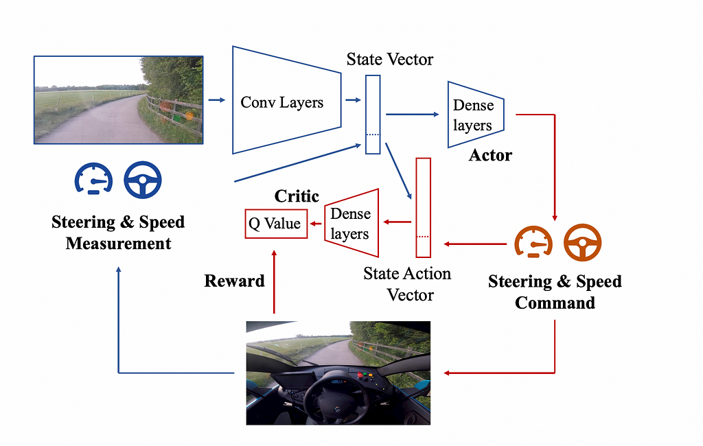
The policy, a strategy the agent uses to decide which action to take in a given state. In deep reinforcement learning, the policy is governed by a deep neural network, in this case a deep deterministic policy gradients (DDPG). This is an off-the-shelf reinforcement learning algorithm with no task-specific adaptation. It is also known as the actor network.
The value function, the estimator of the expected reward the agent can achieve from a given state (or state-action pair). Also known as a critic network. The critic helps guide the actor by providing feedback on the quality of actions during training.
The actor-critic algorithm used to learn a policy and value function for driving from Learning to Drive in a Day
These pieces come together through an iterative learning process. The agent uses its policy to take actions in the environment, observes the resulting state and reward, and updates both the policy (via the actor) and the value function (via the critic). Here’s how it works step-by-step:
Initialization: The agent starts with a randomly initialized policy (actor network) and value function (critic network). It has no prior knowledge of how to drive.
Exploration: The agent explores the environment by taking actions that include some randomness (exploration noise). This ensures the agent tries a wide range of actions to learn their effects, while terrifying regulators.
State Transition: Based on the agent’s action, the environment responds, providing a new state (e.g., the next camera image, speed, and steering angle) and a reward (e.g., the distance traveled without intervention or driving infraction).
Reward Evaluation: The agent evaluates the quality of its action by observing the reward. Positive rewards encourage desirable behaviors (like staying in the lane), while sparse or no rewards prompt improvement.
Learning Update: The agent uses the reward and the observed state transition to update its neural networks:
Critic Network (Value Function): The critic updates its estimate of the Q-function (the function which estimates the reward given an action and state), minimizing the temporal difference (TD) error to improve its prediction of long-term rewards.
Actor Network (Policy): The actor updates its policy by using feedback from the critic, gradually favoring actions that the critic predicts will yield higher rewards.
6. Replay Buffer: Experiences (state, action, reward, next state) are stored in a replay buffer. During training, the agent samples from this buffer to update its networks, ensuring efficient use of data and stability in training.
7. Iteration: The process repeats over and over. The agent refines its policy and value function through trial and error, gradually improving its driving ability.
8. Evaluation: The agent’s policy is tested without exploration noise to evaluate its performance. In Kendall’s work, this meant assessing the car’s ability to stay in the lane and maximize the distance traveled autonomously.
Getting in a car and driving with randomly initialized weights seems a bit daunting! Luckily, what Kendall’s team realized hyper-parameters can be tuned in 3D simulations before being transferred to the real world. They built a simulation engine in Unreal Engine 4 and then ran a generative model for country roads, varied weather conditions and road textures to create training simulations. This vital tuned reinforcement learning parameters like learning rates, number of gradient steps. It also confirmed that a continuous action space was preferable to a discrete one and that DDPG was an appropriate algorithm for the problem.
One of the most interesting aspects of this was how generalized it is versus the mainstream approach. The algorithms and sensors employed are much less specialized than those required by the approaches from companies like Cruise and Waymo. It doesn’t require advancing mapping data or LIDAR data which could make it scalable to new roads and unmapped rural areas.
On the other hand, some downsides of this approach are:
Sparse Rewards. We don’t often fail to stay in the lane, which means the reward only comes from staying in the lane for a long time.
Delayed Rewards. Imagine getting on the George Washington Bridge, you need to pick a lane long before you get on the bridge. This delays the reward making it harder for the model to associate actions and rewards.
High Dimensionality. Both the state space and available actions have a number of dimensions. With more dimensions, the RL model is prone to overfitting or instability due to the sheer complexity of the data.
That being said, Kendall’s team’s achievement is an encouraging step towards autonomous driving. Their goal of lane following was intentionally simplified and illustrates the ease at with RL could be incorperated to help solve the self driving problem. Now lets turn to how it can be applied in labs.
Self-Driving Labs (SDLs)
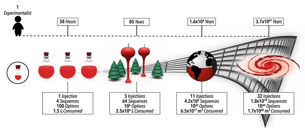
The creators of AlphaFlow argue that much like Kendall’s assessment of driving, that development of lab procotols are a Markov Decision Problem. While Kendall constrained the problem to lane-following, the AlphaFlow team constrained their SDL problem to the optimization of multi-step chemical processes for shell-growth of core-shell semiconductor nanoparticles. Semiconductor nanoparticles have a wide range of applications in solar energy, biomedical devices, fuel cells, environmental remediation, batteries, etc. Methods for discovering types of these materials are typically time-consuming, labor-intensive, and resource-intensive and subject to the curse of dimensionality, the exponential increase in a parameter space size as the dimensionality of a problem increases.
Their RL based approach, AlphaFlow, successfully identified and optimized a novel multi-step reaction route, with up to 40 parameters, that outperformed conventional sequences. This demonstrates how closed-loop RL based approaches can accelerate fundamental knowledge.
Colloidal atomic layer deposition (cALD) is a technique used to create core-shell nanoparticles. The material is grown in a layer-by-layer manner on colloidal particles or quantum dots. The process involves alternating reactant addition steps, where a single atomic or molecular layer is deposited in each step, followed by washing to remove excess reagents. The outcomes of steps can vary due to hidden states or intermediate conditions. This variability reinforces the belief that this as a Markov Decision Problem.
Additionally, the layer-by-layer manner aspect of the technique makes it well suited to an RL approach where we need clear definitions of the state, available actions, and rewards. Furthermore, the reactions are designed to naturally stop after forming a single, complete atomic or molecular layer. This means the experiment is highly controllable and suitable for tools like micro-droplet flow reactors.
Here is how the components of reinforcement learning are mapped to the self driving lab problem:
The agent A decides the next chemical step (either a new surface reaction, ligand addition, or wash step)
The environment is a high-efficiency micro-droplet flow reactor that autonomously conducts experiments.
The state S represents the current setup of reagents, reaction parameters, and short-term memory (STM). In this example, the STM consists of the four prior injection conditions.
The actions A arechoices like reagent addition, reaction timing, and washing steps.
The reward is the in situ optically measured characteristics of the product.
The policy and value function are the RL algorithm which predicts the expected reward and optimizes future decisions. In this case, a belief network composed of an ensemble neural network regressor (ENN) and a gradient-boosted decision tree that classifies the state-action pairs as either viable or unviable.
The rollout policy uses the belief model to predict the outcome/reward of hypothetical future action sequences and decides the next best action to take using a decision policy applied across all predicted action sequences.
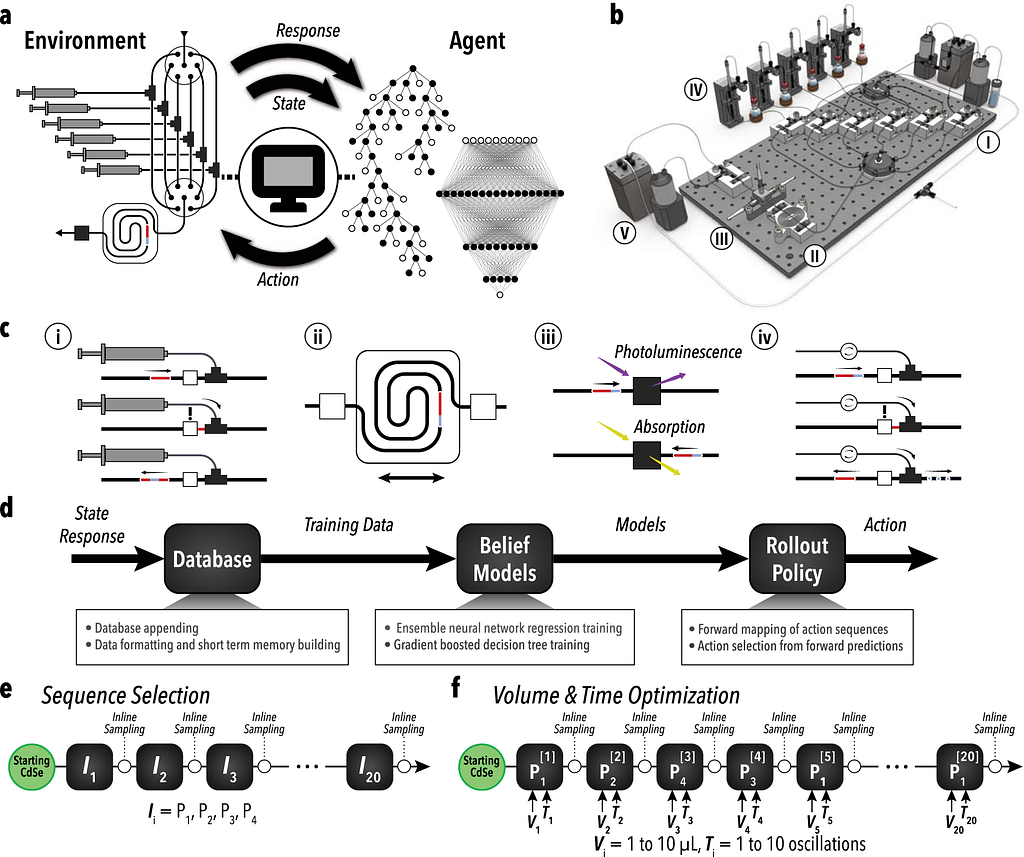
Illustration of the AlphaFlow system and workflow. (a) RL-based feedback loop between the learning agent and the automated experimental setup. (b) Schematic of the reactor system with key modules: reagent injection, droplet mixing, optical sampling, phase separation, waste collection, and refill. (c ) Breakdown of core module functions: formulation, synthesis, characterization, and phase separation. (d) Flow diagram showing how the learning agent selects conditions. (e, f) Overview of reaction space exploration and optimization: sequence selection of reagent injections (P1: oleylamine, P2: sodium sulfide, P3: cadmium acetate, P4: formamide) and volume-time optimization based on the learned sequence.
Similar to the usage of the Unreal Engine by Kendall’s team, the AlphaFlow team used a digital twin structure to help pre-train hyper-parameters before conducting physical experiments. This allowed the model to learn through simulated computational experiments and explore in a more cost efficient manner.
Their approach successfully explored and optimized a 40-dimensional parameter space showcasing how RL can be used to solve complex, multi-step reactions. This advancement could be critical for increasing the throughput experimental validation and helping us unlock advances in a range of fields.
Conclusion
In this post, we explored how reinforcement learning can be applied for self driving and automating lab work. While there are challenges, applications in both domains show how RL can be useful for automation. The idea of furthering fundamental knowledge through RL is of particular interest to the author. I look forward to learning more about emerging applications of reinforcement learning in self driving labs.
We use cookies on our website to give you the most relevant experience by remembering your preferences and repeat visits. By clicking “Accept”, you consent to the use of ALL the cookies.
This website uses cookies to improve your experience while you navigate through the website. Out of these, the cookies that are categorized as necessary are stored on your browser as they are essential for the working of basic functionalities of the website. We also use third-party cookies that help us analyze and understand how you use this website. These cookies will be stored in your browser only with your consent. You also have the option to opt-out of these cookies. But opting out of some of these cookies may affect your browsing experience.
Necessary cookies are absolutely essential for the website to function properly. These cookies ensure basic functionalities and security features of the website, anonymously.
Cookie
Duration
Description
cookielawinfo-checkbox-analytics
11 months
This cookie is set by GDPR Cookie Consent plugin. The cookie is used to store the user consent for the cookies in the category "Analytics".
cookielawinfo-checkbox-functional
11 months
The cookie is set by GDPR cookie consent to record the user consent for the cookies in the category "Functional".
cookielawinfo-checkbox-necessary
11 months
This cookie is set by GDPR Cookie Consent plugin. The cookies is used to store the user consent for the cookies in the category "Necessary".
cookielawinfo-checkbox-others
11 months
This cookie is set by GDPR Cookie Consent plugin. The cookie is used to store the user consent for the cookies in the category "Other.
cookielawinfo-checkbox-performance
11 months
This cookie is set by GDPR Cookie Consent plugin. The cookie is used to store the user consent for the cookies in the category "Performance".
viewed_cookie_policy
11 months
The cookie is set by the GDPR Cookie Consent plugin and is used to store whether or not user has consented to the use of cookies. It does not store any personal data.
Functional cookies help to perform certain functionalities like sharing the content of the website on social media platforms, collect feedbacks, and other third-party features.
Performance cookies are used to understand and analyze the key performance indexes of the website which helps in delivering a better user experience for the visitors.
Analytical cookies are used to understand how visitors interact with the website. These cookies help provide information on metrics the number of visitors, bounce rate, traffic source, etc.
Advertisement cookies are used to provide visitors with relevant ads and marketing campaigns. These cookies track visitors across websites and collect information to provide customized ads.