With access to a wide range of generative AI foundation models (FM) and the ability to build and train their own machine learning (ML) models in Amazon SageMaker, users want a seamless and secure way to experiment with and select the models that deliver the most value for their business. In the initial stages of an ML […]
Evaluating the current LLM landscape based both benchmarks and real-world insights to help you make informed choices.
Image generated by Flux.1 – Schnell
The landscape of Large Language Models (LLMs) for coding has never been more competitive. With major players like Alibaba, Anthropic, Google, Meta, Mistral, OpenAI, and xAI all offering their own models, developers have more options than ever before.
But how can you choose the best LLM for your coding use case?
In this post, I provide an in-depth analysis of the top LLMs available through public APIs. I focus on their performance in coding tasks as measured by benchmarks like HumanEval, and their observed real-world performance as reflected by their respective Elo scores.
Whether you’re working on a personal project or integrating AI into your development workflow, understanding the strengths and weaknesses of these models will help you make a more informed decision.
Disclaimer: challenges when comparing LLMs
Comparing LLMs is hard. Models frequently receive updates that have a significant influence on their performance — say for example OpenAI’s updates from GPT-4 to GPT-4-turbo to GPT-4o to the o1 models. However, even minor updates have an effect — GPT-4o, for example, received already 3 updates after its release on May 13th!
Additionally, the stochastic nature of these models means their performance can vary across different runs, leading to inconsistent results in studies. Finally, some companies may tailor benchmarks and configurations — such as specific Chain-of-Thought techniques — to showcase their models in the best light, which skew comparisons and mislead conclusions.
Conclusion: comparing LLM performance is hard.
This post represents a best-effort comparison of various models for coding tasks based on the information available. I welcome any feedback to improve the accuracy of this analysis!
Evaluating LLMs: HumanEval and Elo scores
As hinted at in the disclaimer above, to properly understand how LLMs perform in coding tasks, it’s advisable to evaluate them from multiple perspectives.
Benchmarking through HumanEval
Initially, I tried to aggregate results from several benchmarks to see which model comes out on top. However, this approach had as core problem: different models use different benchmarks and configurations. Only one benchmark seemed to be the default for evaluating coding performance: HumanEval. This is a benchmark dataset consisting of human-written coding problems, evaluating a model’s ability to generate correct and functional code based on specified requirements. By assessing code completion and problem-solving skills, HumanEval serves as a standard measure for coding proficiency in LLMs.
The voice of the people through Elo scores
While benchmarks give a good view of a model’s performance, they should also be taken with a grain of salt. Given the vast amounts of data LLMs are trained on, some of a benchmark’s content (or highly similar content) might be part of that training. That’s why it’s beneficial to also evaluate models based on how well they perform as judged by humans. Elo ratings, such as those from Chatbot Arena (coding only), do just that. These are scores derived from head-to-head comparisons of LLMs in coding tasks, evaluated by human judges. Models are pitted against each other, and their Elo scores are adjusted based on wins and losses in these pairwise matches. An Elo score shows a model’s relative performance compared to others in the pool, with higher scores indicating better performance. For example, a difference of 100 Elo points suggests that the higher-rated model is expected to win about 64% of the time against the lower-rated model.
Current state of model performance
Now, let’s examine how these models perform when we compare their HumanEval scores with their Elo ratings. The following image illustrates the current coding landscape for LLMs, where the models are clustered by the companies that created them. Each company’s best performing model is annotated.
Figure 1: Elo score by HumanEval — colored by company. X- and y-axis ticks show all models released by each company, with the best performing model shown in bold.
OpenAI’s models are at the top of both metrics, demonstrating their superior capability in solving coding tasks. The top OpenAI model outperforms the best non-OpenAI model — Anthropic’s Claude Sonnet 3.5 — by 46 Elo points , with an expected win rate of 56.6% in head-to-head coding tasks , and a 3.9% difference in HumanEval. While this difference isn’t overwhelming, it shows that OpenAI still has the edge. Interestingly, the best model is o1-mini, which scores higher than the larger o1 by 10 Elo points and 2.5% in HumanEval.
Conclusion: OpenAI continues to dominate, positioning themselves at the top in benchmark performance and real-world usage. Remarkably, o1-mini is the best performing model, outperforming its larger counterpart o1.
Other companies follow closely behind and seem to exist within the same “performance ballpark”. To provide a clearer sense of the difference in model performance, the following figure shows the win probabilities of each company’s best model — as indicated by their Elo rating.
Figure 2: Win probability of each company’s best (coding) model — as illustrated by the Elo ratings’ head-to-head battle win probabilities.
Mismatch between benchmark results and real-world performance
From Figure 1, one thing that stands out is the misalignment between HumanEval (benchmark) and the Elo scores (real-world performance). Some models — like Mistral’s Mistral Large — have significantly better HumanEval scores relative to their Elo rating. Other models — like Google’s Gemini 1.5 Pro — have significantly better Elo ratings relative to the HumanEval score they obtain.
It’s hard to know when to trust benchmarks, as the benchmark data might as well be included in the model’s training dataset. This can lead to (overfitted) models that memorize and repeat the answer to a coding question, rather than understand and actually solve the problem.
Similarly, It’s also problematic to take the Elo ratings as a ground truth, given that these are scores obtained by a crowdsourcing effort. By doing so, you add a human bias to the scoring, favoring models that output in a specific style, take a specific approach, … over others, which does not always align with a factually better model.
Conclusion: better benchmark results don’t always reflect better real-world performance. It’s advised to look at both independently.
The following image shows the disagreement between HumanEval and Elo scores. All models are sorted based on their respective scores, ignoring “how much better” one model is compared to another for simplicity. It shows visually which models perform better on benchmarks than in real life and vice-versa.
Figure 3: Misalignment in HumanEval and Elo scores — colored by company. Scores are transformed to ranks for simplicity, going from worst (left) to best (right) on each metric respectively.
Figure 4 further highlights the difference between benchmarking and real-world performance by simplifying the comparison even further. Here, the figure shows the relative difference in rank, indicating when a model is likely overfitting the benchmark or performs better than reported. Some interesting conclusions can be drawn here:
Overfitting on benchmark: Alibaba and Mistral both stick out for systematically creating models that perform better on benchmarks than in real life. Their most recent models, Alibaba’s Qwen 2.5 Coder (-20.0%) and Mistral’s Mistral Large (-11.5%) follow this pattern, too.
Better than reported: Google stands out for producing models that perform significantly better than reported, with its newest Gemini 1.5 Pro model on top with a difference of +31.5%. Their focus on “honest training and evaluation” is evident in their model reporting and the dicision to develop their own Natural2Code benchmark instead of using HumanEval. “Natural2Code is a code generation benchmark across Python, Java, C++, JS, Go . Held out dataset HumanEval-like, not leaked on the web” ~ Google in the Gimini 1.5 release.
Well balanced: It’s very interesting and particular how well and consistently Meta nails the balance between benchmark a real-world performance. Of course, given that the figure displays rank over score, this stability also depends on the performance of other models.
Figure 4: Performance difference going from HumanEval to Elo scores — colored by company. Negative scores indicate better HumanEval than Elo (overfitting on benchmark) where positive scores indicate better Elo than HumanEval (better performing than reported).
Conclusion: Alibaba and Mistral tend to create models that overfit on the benchmark data.
Conclusion: Google’s models are underrated in benchmark results, due to their focus on fair training and evaluation.
Balancing performance and price: the models that provide the best bang for buck
When choosing an LLM as your coding companion, performance isn’t the only factor to consider. Another important dimension to consider is price. This section re-evaluates the different LLMs and compares how well they fare when evaluated on performance — as indicated by their Elo rating — and price.
Before starting the comparison, it’s worth noting of the odd one out: Meta. Meta’s Llama models are open-source and not hosted by Meta themselves. However, given their popularity, I include them. The price attached to these models is the best pay-as-you-go price offered by the big three cloud vendors (Google, Microsoft, Amazon) — which usually comes down to AWS’s price.
Figure 5 compares the different models and shows the Pareto front. Elo ratings are used to represent model performance, this seemed the best choice given it’s evaluated by humans and doesn’t include an overfitting bias. Next, the pay-as-you-go API price is used with the displayed price being the average of input- and output-token cost for a total of one million generated tokens.
Figure 5: Model coding performance (Elo rating) by API price — colored by company. The models that make up the Pareto front are annotated.
The Pareto front is made up of models coming from only two companies: OpenAI and Google. As mentioned in the previous sections, OpenAI’s models dominate in performance, and they appear to be fairly priced too. Meanwhile, Google seems to focus on lighter weight — thus cheaper — models that still perform well. This makes sense, given their focus on on-device LLM use-cases which hold great strategic value for their mobile operating system (Android).
Conclusion: the Pareto front is made up of models coming from either OpenAI (high performance) or Google (good value for money).
The next figure shows a similar trend when using HumanEval instead of Elo scores to represent coding performance. Some observations:
Anthropic’s Claude 3.5 Haiku is the only notable addition, as this model does not yet have an Elo rating. Could it be a potential contender for middle-priced, high-performance models?
The differences for Google’s Gemini 1.5 Pro and Mistral’s Mistral Large are explained in the previous section that compared HumanEval scores with Elo ratings.
Given that Google’s Gemini 1.5 Flash 8B does not have a HumanEval score, it is excluded from this figure.
Figure 6: Model coding performance (HumanEval score) by API price — colored by company. The models that make up the Pareto front are annotated.
Shifting through the data: additional insights and trends
To conclude, I will discuss some extra insights worth noting in the current LLM (coding) landscape. This section explores three key observations: the steady improvement of models over time, the continued dominance of proprietary models, and the significant impact even minor model updates can have. All the observations stem from the Elo rating by price comparison shown in Figure 5.
Models are getting better and cheaper
The following figure illustrates how new models continue to achieve higher accuracy while simultaneously driving down costs. It’s remarkable to see how three time segments — 2023 and before, H1 of 2024, and H2 of 2024 — each define their own Pareto front and occupy almost completely distinct segments. Curious to see how this will continue to progress in 2025!
Figure 7: Evolution of time as indicated by three different time segments — 2023 and before, H1 of 2024, and H2 of 2024.
Conclusion: models get systematically better and cheaper, a trend observed with almost every new model release.
Proprietary models remain in power
The following image shows which of the analyzed models are proprietary and which are open-source. We see that proprietary models continue to dominate the LLM coding landscape. The Pareto front is still driven by these “closed-source” models, both on the high-performing and low-cost ends.
However, open-source models are closing the gap. It’s interesting to see, though, that for each open-source model, there is a proprietary model with the same predictive performance that is significantly cheaper. This suggests that the proprietary are either more lighterweight or better optimized, thus requiring less computational power — though this is just a personal hunch.
Figure 8: Proprietary versus open-source models.
Conclusion: proprietary models continue to hold the performance-cost Pareto front.
Even minor model updates have an effect
The following and final image illustrates how even minor updates to the same models can have an impact. Most often, these updates bring a performance boost, improving the models gradually over time without a major release. Occasionally though, a model’s performance might drop for coding tasks following a minor update, but this is almost always accompanied by a reduction in price. This is likely because the models were optimized in some way, such as through quantization or pruning parts of their network.
Figure 9: Evolution of model performance and price for minor model updates.
Conclusion: minor model updates almost always improve performance or push down cost.
Conclusion: key takeaways of LLMs for coding
The LLM landscape for coding is rapidly evolving, with newer models regularly pushing the Pareto front toward better-performing and/or cheaper options. Developers must stay informed about the latest models to identify those that offer the best capabilities within their budget. Recognizing the misalignment between real-world results and benchmarks is essential to making informed decisions. By carefully weighing performance against cost, developers can choose the tools that best meet their needs and stay ahead in this dynamic field.
Here’s a quick overview of all the conclusions made in this post:
Comparing LLM performance is hard.
OpenAI continues to dominate, positioning themselves at the top in benchmark performance and real-world usage. Remarkably, o1-mini is the best performing model, outperforming its larger counterpart o1.
Better benchmark results don’t always reflect better real-world performance. It’s advised to look at both independently.
Alibaba and Mistral tend to create models that overfit on the benchmark data.
Google’s models are underrated in benchmark results, due to their focus on fair training and evaluation.
The Pareto front is made up of models coming from either OpenAI (high performance) or Google (good value for money).
Models get systematically better and cheaper, a trend observed with almost every new model release.
Proprietary models continue to hold the performance-cost Pareto front.
Minor model updates almost always improve performance or push down cost.
Found this useful? Feel free to follow me on LinkedIn to see my next explorations!
The images shown in this article were created by myself, the author, unless specified otherwise.
Are LLMs Better at Generating SQL, SPARQL, Cypher, or MongoDB Queries?
Our NeurIPS’24 paper sheds light on this underinvestigated topic with a new and unique public dataset and benchmark.
(Image by author)
Many recent works have been focusing on how to generate SQL from a natural language question using an LLM. However, there is little understanding of how well LLMs can generate other database query languages in a direct comparison. To answer the question, we created a completely new dataset and benchmark of 10K question-query pairs covering four databases and query languages. We evaluated several relevant closed and open-source LLMs from OpenAI, Google, and Meta together with common in-context-learning (ICL) strategies. The corresponding paper “SM3-Text-to-Query: Synthetic Multi-Model Medical Text-to-Query Benchmark” [1] is published at NeurIPS 2024 in the Dataset and Benchmark track (https://arxiv.org/abs/2411.05521). All code and data are available at https://github.com/jf87/SM3-Text-to-Query to enable you to test your own Text-to-Query method across four query languages. But before we look at Text-to-Query, let’s first take a step back and examine the more common paradigm of Text-to-SQL.
What is Text-to-SQL?
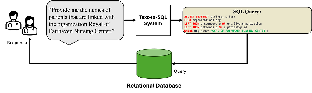
Text-to-SQL (also called NL-to-SQL) systems translate the provided natural language question into a corresponding SQL query. SQL has served as a primary query language for structured data sources (relational model), offering a declarative interface for application developers to access information. Text-to-SQL systems thus aim to enable non-SQL expert users to access and fulfill their information needs by simply making their requests in natural language.
Figure 1. Overview Text-to-SQL. Users ask questions in natural language, which are then translated to the corresponding SQL query. The query is executed against a relational database such as PostgreSQL, and the response is returned to the users. (Image by author)
Text-to-SQL methods have recently increased in popularity and made substantial progress in terms of their generation capabilities. This can easily be seen from Text-to-SQL accuracies reaching 90% on the popular benchmark Spider (https://yale-lily.github.io/spider) and up to 74% on the more recent and more complex BIRD benchmark (https://bird-bench.github.io/). At the core of this success lie the advancements in transformer-based language models, from Bert [2] (340M parameters) and Bart [ 3 ] (148M parameters) to T5 [4 ] (3B parameters) to the advent of Large Language Models (LLMs), such as OpenAI’s GPT models, Anthropic Claude models or Meta’s LLaMA models (up to 100s of billions of parameters).
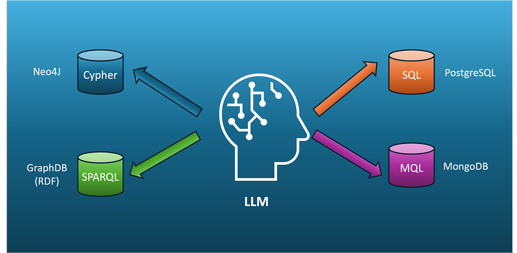
Beyond Relational Databases: Document & Graph Model
While many structured data sources inside companies and organizations are indeed stored in a relational database and accessible through the SQL query language, there are other core database models (also often referred to as NoSQL) that come with their own benefits and drawbacks in terms of ease of data modeling, query performance, and query simplicity:
Relational Database Model. Here, data is stored in tables (relations) with a fixed, hard-to-evolve schema that defines tables, columns, data types, and relationships. Each table consists of rows (records) and columns (attributes), where each row represents a unique instance of the entity described by the table (for example, a patient in a hospital), and each column represents a specific attribute of that entity. The relational model enforces data integrity through constraints such as primary keys (which uniquely identify each record) and foreign keys (which establish relationships between tables). Data is accessed through SQL. Popular relational databases include PostgreSQL, MySQL, and Oracle Database.
Document Database Model. Here, data is stored in a document structure (hierarchical data model) with a flexible schema that is easy to evolve. Each document is typically represented in formats such as JSON or BSON, allowing for a rich representation of data with nested structures. Unlike relational databases, where data must conform to a predefined schema, document databases allow different documents within the same collection to have varying fields and structures, facilitating rapid development and iteration. This flexibility means that attributes can be added or removed without affecting other documents, making it suitable for applications where requirements change frequently. Popular document databases include MongoDB, CouchDB, and Amazon DocumentDB.
Graph Database Model. Here, data is represented as nodes (entities) and edges (relationships) in a graph structure, allowing for the modeling of complex relationships and interconnected data. This model provides a flexible schema that can easily accommodate changes, as new nodes and relationships can be added without altering existing structures. Graph databases excel at handling queries involving relationships and traversals, making them ideal for applications such as social networks, recommendation systems, and fraud detection. Popular graph databases include Neo4j, Amazon Neptune, and ArangoDB.
From Text-to-SQL to Text-to-Query
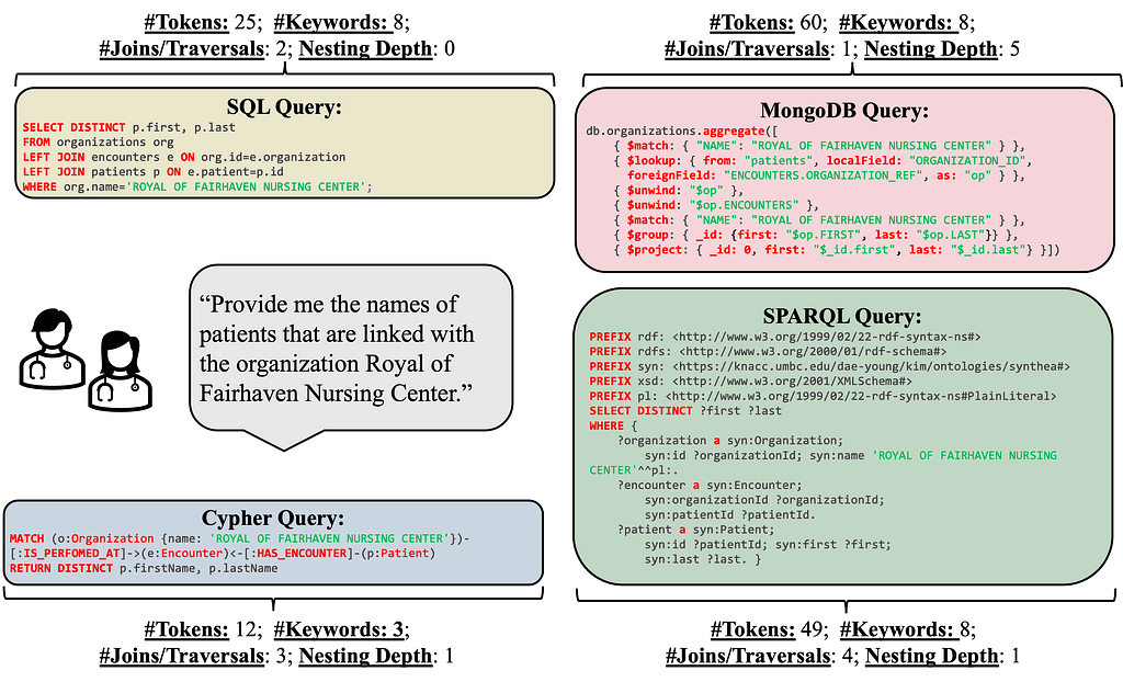
The choice of database and the underlying core data model (relational, document, graph) has a large impact on read/write performance and query complexity. For example, the graph model naturally represents many-to-many relationships, such as connections between patients, doctors, treatments, and medical conditions. In contrast, relational databases require potentially expensive join operations and complex queries. Document databases have only rudimentary support for many-to-many relationships and aim at scenarios where data is not highly interconnected and stored in collections of documents with a flexible schema.
Figure 2. Differences across query languages and database systems for the same user request. (Image by author)
While these differences have been a known fact in database research and industry, their implications for the growing number of Text-to-Query systems have surprisingly not been investigated so far.
SM3-Text-to-Query Benchmark
SM3-Text-to-Query is a new dataset and benchmark that enables the evaluation across four query languages (SQL, MongoDB Query Language, Cypher, and SPARQL) and three data models (relational, graph, document).
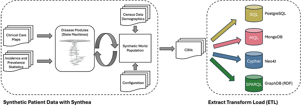
Figure 3. SM3-Text-to-Query Benchmark Construction. Combining synthetic patient data generation with ETL processes for four databases makes it possible to create arbitrarily large synthetic datasets. (Image by author)
SM3-Text-to-Query is constructed from synthetic patient data created with Synthea. Synthea is an open-source synthetic patient generator that produces realistic electronic health record (EHR) data. It simulates patients’ medical histories over time, including various demographics, diseases, medications, and treatments. This created data is then transformed and loaded into four different database systems: PostgreSQL, MongoDB, Neo4J, and GraphDB (RDF).
Based on a set of > 400 manually created template questions and the generated data, 10K question-query pairs are generated for each of the four query languages (SQL, MQL, Cypher, and SPARQL). However, based on the synthetic data generation process, adding additional template questions or generating your own patient data is also easily possible (for example, adapted to a specific region or in another language). It would even be possible to construct a (private) dataset with actual patient data.
Text-to-Query Results
So, how do current LLMs perform in the generation across the four query languages? There are three main lessons that we can learn from the reported results.
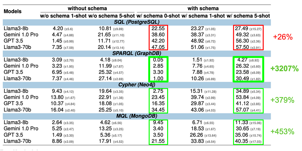
Lesson 01: Schema information helps for all query languages but not equally well.
Schema information helps for all query languages, but its effectiveness varies significantly. Models leveraging schema information outperform those that don’t — even more in one-shot scenarios where accuracy plummets otherwise. For SQL, Cypher, and MQL, it can more than double the performance. However, SPARQL shows only a small improvement. This suggests that LLMs may already be familiar with the underlying schema (SNOMED CT, https://www.snomed.org), which is a common medical ontology.
Figure 4. Impact of Schema Information on Execution Accuracy. (Image by author)
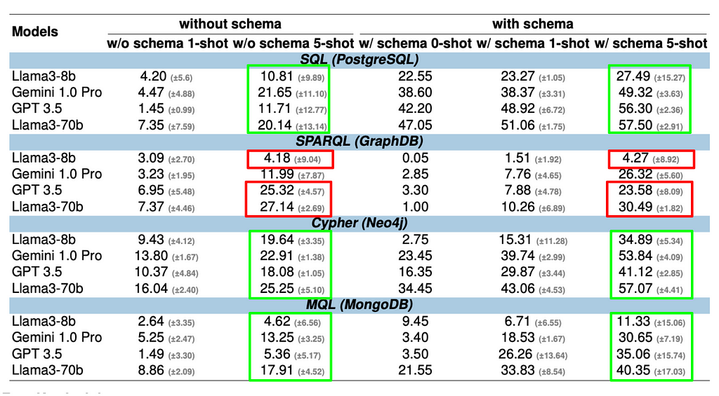
Lesson 02: Adding examples improves accuracy through in-context learning (ICL) for all LLMs and query languages; however, the rate of improvement varies greatly across query languages.
Examples enhance accuracy through in-context learning (ICL) across all LLMs and query languages. However, the degree of improvement varies greatly. For SQL, the most popular query language, larger LLMs (GPT-3.5, Llama3–70b, Gemini 1.0) already show a solid baseline accuracy of around 40% with zero-shot schema input, gaining only about 10% points with five-shot examples. However, the models struggle significantly with less common query languages such as SPARQL and MQL without examples. For instance, SPARQL’s zero-shot accuracy is below 4%. Still, with five-shot examples, it skyrockets to 30%, demonstrating that ICL supports models to generate more accurate queries when provided with relevant examples.
Figure 5. Impact of In-Context-Learning (ICL) through Few-shot Examples. (Image by author)
Lesson 03: LLMs have varying levels of training knowledge across different query languages
LLMs exhibit differing levels of proficiency across query languages. This is likely rooted in their training data sources. An analysis of Stack Overflow posts supports this assumption. There is a big contrast in the post-frequency for the different query languages:
[SQL]: 673K posts
[SPARQL]: 6K posts
[MongoDB, MQL]: 176K posts
[Cypher, Neo4J]: 33K posts
This directly correlates with the zero-shot accuracy results, where SQL leads with the best model accuracy of 47.05%, followed by Cypher and MQL at 34.45% and 21.55%. SPARQL achieves just 3.3%. These findings align with existing research [5], indicating that the frequency and recency of questions on platforms like Stack Overflow significantly impact LLM performance. An intriguing exception arises with MQL, which underperforms compared to Cypher, likely due to the complexity and length of MQL queries.
Conclusion
SM3-Text-to-query is the first dataset that targets the cross-query language and cross-database model evaluation of the increasing number of Text-to-Query systems that are fueled by rapid progress in LLMs. Existing works have mainly focused on SQL. Other important query languages are underinvestigated. This new dataset and benchmark allow a direct comparison of four relevant query languages for the first time, making it a valuable resource for both researchers and practitioners who want to design and implement Text-to-Query systems.
The initial results already provide many interesting insights, and I encourage you to check out the full paper [1].
Try it yourself
All code and data are open-sourced on https://github.com/jf87/SM3-Text-to-Query. Contributions are welcome. In a follow-up post, we will provide some hands-on instructions on how to deploy the different databases and try out your own Text-to-Query method.
[1] Sivasubramaniam, Sithursan, Cedric Osei-Akoto, Yi Zhang, Kurt Stockinger, and Jonathan Fuerst. “SM3-Text-to-Query: Synthetic Multi-Model Medical Text-to-Query Benchmark.” In The Thirty-eight Conference on Neural Information Processing Systems Datasets and Benchmarks Track. [2] Devlin, Jacob. “Bert: Pre-training of deep bidirectional transformers for language understanding.” arXiv preprint arXiv:1810.04805 (2018). [3]Mike Lewis, Yinhan Liu, Naman Goyal, Marjan Ghazvininejad, Abdelrahman Mohamed, Omer Levy, Veselin Stoyanov, and Luke Zettlemoyer. 2020. BART: Denoising Sequence-to-Sequence Pre-training for Natural Language Generation, Translation, and Comprehension. In Proceedings of the 58th Annual Meeting of the Association for Computational Linguistics, pages 7871–7880, Online. Association for Computational Linguistics. [4] Raffel, Colin, Noam Shazeer, Adam Roberts, Katherine Lee, Sharan Narang, Michael Matena, Yanqi Zhou, Wei Li, and Peter J. Liu. “Exploring the limits of transfer learning with a unified text-to-text transformer.” Journal of machine learning research 21, no. 140 (2020): 1–67. [5] Kabir, Samia, David N. Udo-Imeh, Bonan Kou, and Tianyi Zhang. “Is stack overflow obsolete? an empirical study of the characteristics of chatgpt answers to stack overflow questions.” In Proceedings of the CHI Conference on Human Factors in Computing Systems, pp. 1–17. 2024.
What should be done when an AI accuses a student of misconduct by using AI?
Anti-cheating tools that detect material generated by AI systems are widely being used by educators to detect and punish cheating on both written and coding assignments. However, these AI detection systems don’t appear to work very well and they should not be used to punish students. Even the best system will have some non-zero false positive rate, which results in real human students getting F’s when they did in fact do their own work themselves. AI detectors are widely used, and falsely accused students span a range from grade school to grad school.
In these cases of false accusation, the harmful injustice is probably not the fault of the company providing the tool. If you look in their documentation then you will typically find something like:
“The nature of AI-generated content is changing constantly. As such, these results should not be used to punish students. … There always exist edge cases with both instances where AI is classified as human, and human is classified as AI.” — Quoted from GPTZero’s FAQ.
In other words, the people developing these services know that they are imperfect. Responsible companies, like the one quoted above, explicitly acknowledge this and clearly state that their detection tools should not be used to punish but instead to see when it might make sense to connect with a student in a constructive way. Simply failing an assignment because the detector raised a flag is negligent laziness on the part of the grader.
If you’re facing cheating allegations involving AI-powered tools, or making such allegations, then consider the following key questions:
What detection tool was used and what specifically does the tool purport to do? If the answer is something like the text quoted above that clearly states the results are not intended for punishing students, then the grader is explicitly misusing the tool.
In your specific case, is the burden of proof on the grader assigning the punishment? If so, then they should be able to provide some evidence supporting the claim that the tool works. Anyone can make a website that just uses an LLM to evaluate the input in a superficial way, but if it’s going to be used as evidence against students then there needs to be a formal assessment of the tool to show that it works reliably. Moreover this assessment needs to be scientifically valid and conducted by a disinterested third party.
In your specific case, are students entitled to examine the evidence and methodology that was used to accuse them? If so then the accusation may be invalid because AI detection software typically does not allow for the required transparency.
Is the student or a parent someone with English as a second language? If yes, then there may be a discrimination aspect to the case. People with English as second language often directly translate idioms or other common phrases and expressions from their first language. The resulting text ends up with unusual phrases that are known to falsely trigger these detectors.
Is the student a member of a minority group that makes use of their own idioms or English dialect? As with second-language speakers, these less common phrases can falsely trigger AI detectors.
Is the accused student neurodiverse? If yes, then this is another possible discrimination aspect to the case. People with autism, for example, may use expressions that make perfect sense to them, but that others find odd. There is nothing wrong with these expressions, but they are unusual and AI detectors can be triggered by them.
Is the accused work very short? The key idea behind AI detectors is that they look for unusual combinations of words and/or code instructions that are seldom used by humans yet often used by generative AI. In a lengthly work, there may be many such combinations found so that the statistical likelihood of a human coincidentally using all of those combinations could be small. However, the shorter the work, the higher the chance of coincidental use.
What evidence is there that the student did the work? If the assignment in question is more than a couple paragraphs or a few lines of code then it is likely that there is a history showing the gradual development of the work. Google Docs, Google Drive, and iCloud Pages all keep histories of changes. Most computers also keep version histories as part of their backup systems, for example Apple’s Time Machine. Maybe the student emailed various drafts to a partner, parent, or even the teacher and those emails form a record incremental work. If the student is using GitHub for code then there is a clear history of commits. A clear history of incremental development shows how the student did the work over time.
To be clear, I think that these AI detection tools have a place in education, but as the responsible websites themselves clearly state, that role is not to catch cheaters and punish students. In fact, many of these websites offer guidance on how to constructively address suspected cheating. These AI detectors are tools and like any powerful tool they can be great if used properly and very harmful if used improperly.
If you or your child has been unfairly accused of using AI to write for them and then punished, then I suggest that you show the teacher/professor this article and the ones that I’ve linked to. If the accuser will not relent then I suggest that you contact a lawyer about the possibility of bringing a lawsuit against the teacher and institution/school district.
Despite this recommendation to consult an attorney, I am not anti-educator and think that good teachers should not be targeted by lawsuits over grades. However, teachers that misuse tools in ways that harm their students are not good teachers. Of course a well-intentioned educator might misuse the tool because they did not realize its limitations, but then reevaluate when given new information.
“it is better 100 guilty Persons should escape than that one innocent Person should suffer” — Benjamin Franklin, 1785
As a professor myself, and I’ve also grappled with cheating in my classes. There’s no easy solution, and using AI detectors to fail students is not only ineffective but also irresponsible. We’re educators, not police or prosecutors. Our role should be supporting our students, not capriciously punishing them. That includes even the cheaters, though they might perceive otherwise. Cheating is not a personal affront to the educator or an attack on the other students. At the end of the course, the only person truly harmed by cheating is the cheater themself who wasted their time and money without gaining any real knowledge or experience. (Grading on a curve, or in some other way that pits students against each other, is bad for a number of reasons and, in my opinion, should be avoided.)
Finally, AI systems are here to stay and like calculators and computers they will radically change how people work in the near future. Education needs to evolve and teach students how to use AI responsibly and effectively. I wrote the first draft of this myself, but then I asked an LLM to read it, give me feedback, and make suggestions. I could probably have gotten a comparable result without the LLM, but then I would likely have asked a friend to read it and make suggestions. That would have taken much longer. This process of working with an LLM is not unique to me, rather it is widely used by my colleagues. Perhaps, instead of hunting down AI use, we should be teaching it to our students. Certainly, students still need to learn fundamentals, but they also need to learn how to use these powerful tools. If they don’t, then their AI-using colleagues will have a huge advantage over them.
About Me: James F. O’Brien is a Professor of Computer Science at the University of California, Berkeley. His research interests include computer graphics, computer animation, simulations of physical systems, human perception, rendering, image synthesis, machine learning, virtual reality, digital privacy, and the forensic analysis of images and video.
Disclaimer: Any opinions expressed in this article are only those of the author as a private individual. Nothing in this article should be interpreted as a statement made in relation to the author’s professional position with any institution.
This article and all embedded images are Copyright 2024 by the author. This article was written by a human, and both an LLM (Llama 3.2 3B) and other humans were used for proofreading and editorial suggestions. The editorial image was generated by AI (Adobe Firefly) and then substantially edited by a human using Photoshop.
Finding customer segments for optimal retargetting using LLM embeddings and ML model
Introduction
In this article, we are talking about a method of finding the customer segments within a binary classification dataset which have the maximum potential to tip over into the wanted class. This method can be employed for different use-cases such as selective targetting of customers in the second round of a promotional campaign, or finding nodes in a network, which are providing less-than-desirable experience, with the highest potential to move over into the desirable category.
Essentially, the method provides a way to prioritise a segment of the dataset which can provide the maximum bang for the buck.
The context
In this case, we are looking at a bank dataset. The bank is actively trying to sell loan products to the potential customers by runnign a campaign. This dataset is in public domain provided at Kaggle:
The description of the problem given above is as follows:
“The majority of Thera-Bank’s customers are depositors. The number of customers who are also borrowers (asset customers) is quite small, and the bank is interested in quickly expanding this base to do more loan business while earning more through loan interest. In particular, management wants to look for ways to convert its liability customers into retail loan customers while keeping them as depositors. A campaign the bank ran last year for deposit customers showed a conversion rate of over 9.6% success. This has prompted the retail marketing department to develop campaigns with better target marketing to increase the success rate with a minimal budget.”
The above problem deals with classifying the customers and helping to prioritise new customers. But what if we can use the data collected in the first round to target customers who did not purchase the loan in the first round but are most likely to purchase in the second round, given that at least one attribute or feature about them changes. Preferably, this would be the feature which is easiest to change through manual interventions or which can change by itself over time (for example, income generally tends to increase over time or family size or education level attained).
The Solution
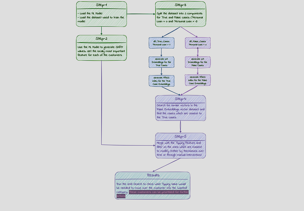
Here is an overview of how this problem is approached in this example:
High Level Process Flow
Step -1a : Loading the ML Model
There are numerous notebooks on Kaggle/Github which provide solutions to do model tuning using the above dataset. We will start our discussion with the assumption that the model is already tuned and will load it up from our MLFlow repository. This is a XGBoost model with F1 Score of 0.99 and AUC of 0.99. The dependent variable (y_label) in this case is ‘Personal Loan’ column.
def get_best_model(experiment_name, scoring_metric): """ Retrieves the model from MLflow logged models in a given experiment with the best scoring metric.
Args: experiment_name (str): Name of the experiment to search. scoring_metric (str): f1_score is used in this example
Returns: model_uri: The model path with the best F1 score, or None if no model or F1 score is found. artifcat_uri: The path for the artifacts for the best model """ experiment = mlflow.get_experiment_by_name(experiment_name)
# Extract the experiment ID if experiment: experiment_id = experiment.experiment_id print(f"Experiment ID for '{experiment_name}': {experiment_id}") else: print(f"Experiment '{experiment_name}' not found.")
client = mlflow.tracking.MlflowClient()
# Find runs in the specified experiment runs = client.search_runs(experiment_ids=experiment_id)
# Initialize variables for tracking best_run = None best_score = -float("inf") # Negative infinity for initial comparison
for run in runs: try: run_score = float(run.data.metrics.get(scoring_metric, 0)) # Get F1 score from params if run_score > best_score: best_run = run best_score = run_score Model_Path = best_run.data.tags.get("Model_Type")
except (KeyError): # Skip if score not found or error occurs pass
# Return the model version from the run with the best F1 score (if found) if best_run:
model_uri = f"runs:/{best_run.info.run_id}/{Model_Path}" artifact_uri = f"mlflow-artifacts:/{experiment_id}/{best_run.info.run_id}/artifacts" print(f"Best Score found for {scoring_metric} for experiment: {experiment_name} is {best_score}") print(f"Best Model found for {scoring_metric} for experiment: {experiment_name} is {Model_Path}") return model_uri, artifact_uri
else: print(f"No model found with logged {scoring_metric} for experiment: {experiment_name}") return None
if best_model_uri: loaded_model = mlflow.sklearn.load_model(best_model_uri)
Step-1b: Loading the data
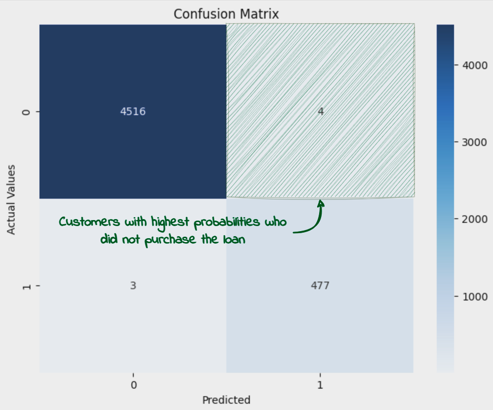
Next, we would load up the dataset. This is the dataset which has been used for training the model, which means all the rows with missing data or the ones which are considered outliers are already removed from the dataset. We would also calculate the probabilities for each of the customers in the dataset to purchase the loan (given by the column ‘Personal Loan). We will then filter out the customers with probabilities greater than 0.5 but which did not purchase the loan (‘Personal Loan’ = 0). These are the customers which should have purchased the Loan as per the prediction model but they did not in the first round, due to factors not captured by the features in the dataset. These are also the cases wrongly predicted by the model and which have contributed to a lower than 1 Accuracy and F1 figures.
Confusion Matrix
As we set out for round 2 campaign, these customers would serve as the basis for the targetted marketing approach.
import numpy as np import pandas as pd import os
y_label_column = "Personal Loan"
def y_label_encoding (label):
try:
if label == 1: return 1 elif label == 0: return 0 elif label == 'Yes': return 1 elif label == 'No': return 0 else: print(f"Invalid label: {label}. Only 'Yes/1' or 'No/0' are allowed.") except: print('Exception Raised')
load_prediction_data function should refer to the final dataset used for training. The function is not provided here
"""
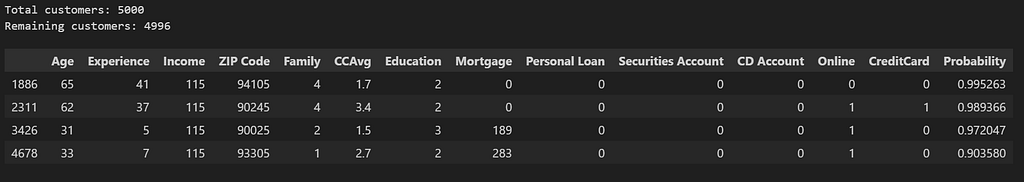
df_pred = load_prediction_data (best_artifact_uri) ##loads dataset into a dataframe df_pred['Probability'] = [x[1] for x in loaded_model.predict_proba(df_splitting(df_pred)[0])] df_pred = df_pred.sort_values(by='Probability', ascending=False) df_potential_cust = df_pred[(df_pred[y_label_column]==0) & (df_pred['Probability']> 0.5)] print(f'Total customers: {df_pred.shape[0]}') df_pred = df_pred[~((df_pred[y_label_column]==0) & (df_pred['Probability']> 0.5))] print(f'Remaining customers: {df_pred.shape[0]}') df_potential_cust
We see that there are only 4 such cases which get added to potential customers table and are removed from the main dataset.
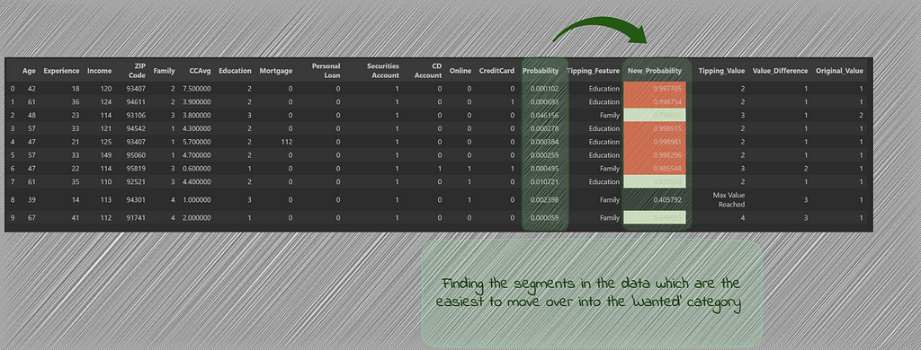
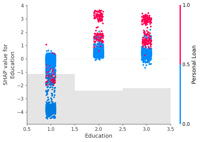
Step-2: Generating SHAP values
We are now going to generate the Shapely values to determine the local importance of the features and extract the Tipping feature ie. the feature whose variation can move over the customer from unwanted class (‘Personal Loan’ = 0) to the wanted class (‘Personal Loan’ = 1). Details about Shapely values can be found here:
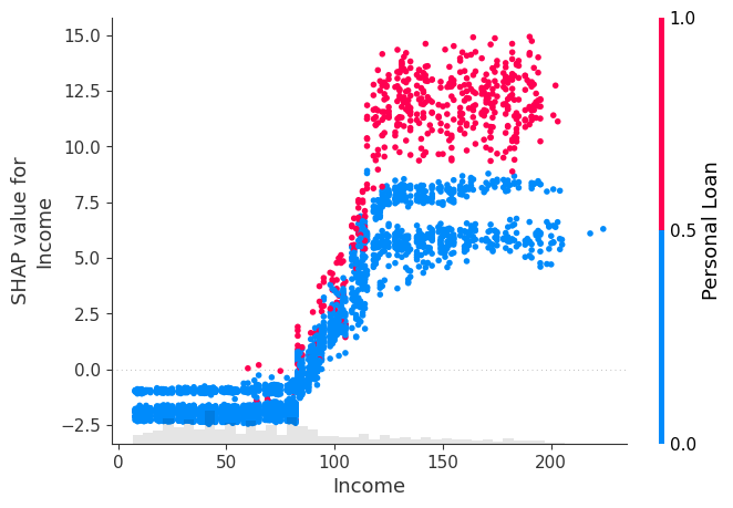
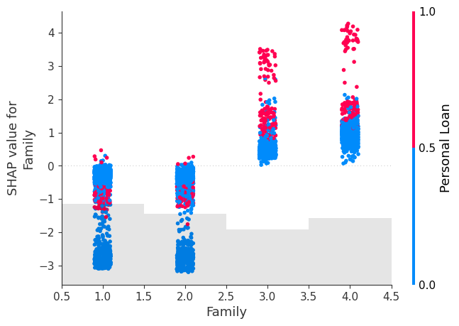
We will have a look at some of the important features as well to have an idea about the correlation with the dependent variable (‘Personal Loan’). The three features we have shortlisted for this purpose are ‘Income’, ‘Family’ (Family Size) and ‘Education’. As we will see later on, these are the features which we would want to keep our focus on to get the probability changed.
Purchase of Personal Loan increases with Education
We see that for all 3 features, the purchase of Personal Loan increase as the feature value tends to increase, with Shap values of greater than 0 as the feature value increases indicating a positive impact of these features on the tendency to purchase.
We will now store the shap values for each of the customers in a dataframe so we can access the locally most important feature for later processing.
X_test = df_splitting(df_pred)[0] ## Keeping only the columns used for prediction
explainer = shap.Explainer(loaded_model.predict, X_test)
Shap_explainer = explainer(X_test)
df_Shap_values = pd.DataFrame(Shap_explainer.values, columns=X_test.columns)
df_Shap_values.to_csv('Credit_Card_Fraud_Shap_Values.csv', index=False)
Step-3 : Creating Vector Embeddings:
As the next step, we move on to create the vector embeddings for our dataset using LLM model. The main purpose for this is to be able to do vector similarity search. We intend to find the customers in the dataset, who did not purchase the loan, who are closest to the customers in the dataset, who did purchase the loan. We would then pick the top closest customers and see how the probability changes for these once we change the values for the most important feature for these customers.
There are a number of steps involved in creating the vector embeddings using LLM and they are not described in detail here. For a good understanding of these processes, I would suggest to go through the below post by Damian Gill:
For us to get better vector embeddings, we would want to provide as much details about the data in words as possible. For the bank dataset, the details of each of the columns are provided in ‘Description’ sheet of the Excel file ‘Bank_Personal_Loan_Modelling.xlsx’. We use this description for the column names. Additionally, we convert the values with a little more description than just having numbers in there. For example, we replace column name ‘Family’ with ‘Family size of the customer’ and the values in this column from integers such as 2 to string such as ‘2 persons’. Here is a sample of the dataset after making these conversions:
if row.sum() < 0: top_values = row.nsmallest(no_of_values) else: top_values = row.nlargest(no_of_values) return [f"{col}: {val}" for col, val in zip(top_values.index, top_values)]
Original_Categorized_Dataset = r'Bank_Personal_Loan_Modelling_Semantic.csv' ## Dataset with more description of the values sorted in the same way as df_pred and df_Shap_values Shap_values_Dataset = r'Credit_Card_Fraud_Shap_Values.csv' ## Shap values dataset column_description = r'Bank_Personal_Loan_Modelling.xlsx' ## Original Bank Loan dataset with the Description Sheet
We will create two separate datasets — one for customers who purchased the loans and one for those who didn’t.
y_label_column = 'Did this customer accept the personal loan offered in the last campaign?'
df_main_true_cases = df_main[df_main[y_label_column]=="Yes"].reset_index(drop=True)
df_main_false_cases = df_main[df_main[y_label_column]=="No"].reset_index(drop=True)
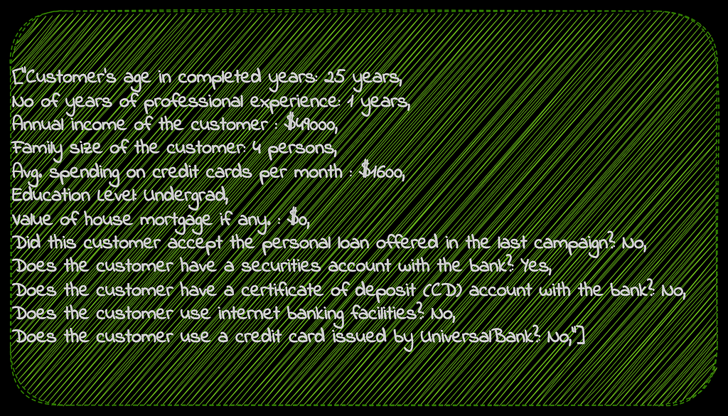
We will create vector embeddings for both of these cases. Before we pass on the dataset to sentence transformer, here is what each row of the bank customer dataset would look like:
Example of one customer input to Sentence Transformer
from sentence_transformers import SentenceTransformer
def df_to_text(row):
text = '' for col in row.index: text += f"""{col}: {row[col]},""" return text
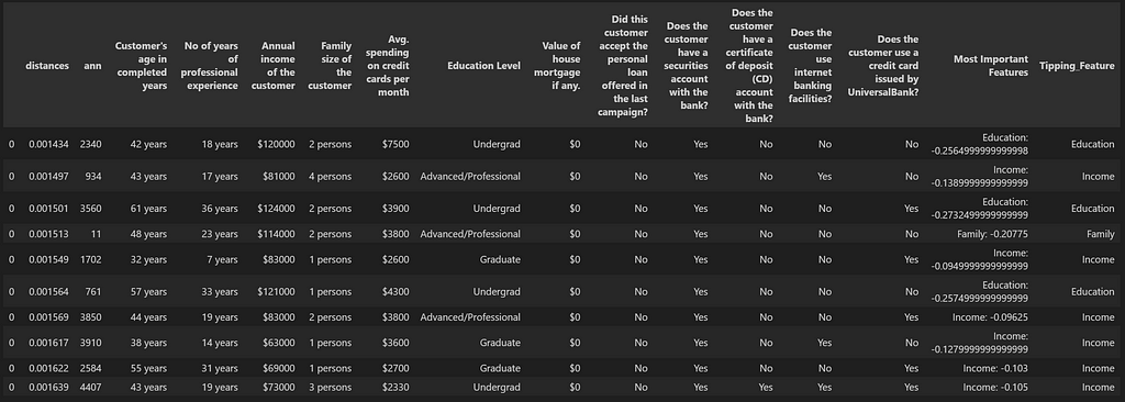
Next, we will be doing the Approximate Nearest Neighbor similarity search using Euclidean Distance L2 with Facebook AI Similarity Search (FAISS) and will create FAISS indexes for these vector datasets. The idea is to search for customers in the ‘Personal Loan = 0’ dataset which are most similar to the ones in the ‘Personal Loan = 1’ dataset. Basically we are looking for customers who did not purchase the loan but are most similar in nature to the ones who purchased the loan. In this case, we are doing the search for one ‘false’ customer for each ‘true’ customer by setting k=1 (one approximate nearest neighbor) and then sorting the results based on their distances.
Details about FAISS similarity search can be found here:
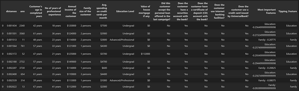
df_results = cluster_search(index_false_cases, df_embedding_true_cases, df_main_false_cases, k=1) df_results['Most Important Features'] = [x[0] for x in df_results['Most Important Features'].values] df_results ['Tipping_Feature'] = [x[0] for x in df_results['Most Important Features'].str.split(':')] df_results = df_results.drop_duplicates(subset=['ann']) df_results.head(10)
This gives us the list of customers most similar to the ones who purchased the loan and most likely to purchase in the second round, given the most important feature which was holding them back in the first round, gets slightly changed. This customer list can now be prioritized.
Step-6: A comparison with other method
At this point, we would like to assess if the above methodology is worth the time and if there can be another efficient way of extracting the same information? For example, we can think of getting the ‘False’ customers with the highest probabilities as the ones which have the highest potential for second round purchases. A comparison of such a list with the above list can be helpful to see if that can be a faster way of deriving conclusions.
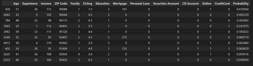
For this, we simply load up our dataset with the probabilities that we created earlier and pick the top 10 ‘False’ customers with the highest probabilities.
How effective this list is as compared to our first list and how to measure that? For this, we would like to think of the effectiveness of the list as the percentage of customers which we are able to tip over into the wanted category with minimal change in the most important feature by calculating new probability values after making slight change in the most important feature. For our analysis, we will only focus on the features Education and Family — the features which are likely to change over time. Even though Income can also be included in this category, for simplification purposes, we will not consider it for now. We will shortlist the top 10 candidates from both lists which have these as the Tipping_Feature.
This will give us the below 2 lists:
List_A: This is the list we get using the similarity search method
List_B: This is the list we get through sorting the False cases using their probabilities
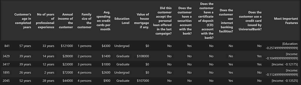
We will convert List_A into the original format which can be then used by the ML Model to calculate the probabilities. This would require a reference back to the original df_pred dataset and here is a function which can be used for that purpose.
Potential Candidates List_A: Extracted using the similarity Search method
Below is how we will get List_B by putting in the required filters on the original df_pred dataframe.
df_list_B_Probabilities = df_pred.copy().reset_index(drop=True)
df_list_B_Probabilities['Tipping_Feature'] = df_Shap_values.apply(lambda row: Get_Highest_SHAP_Values(row, no_of_values = 1), axis=1)
df_list_B_Probabilities['Tipping_Feature'] = [x[0] for x in df_list_B_Probabilities['Tipping_Feature'].values]
df_list_B_Probabilities ['Tipping_Feature'] = [x[0] for x in df_list_B_Probabilities['Tipping_Feature'].str.split(':')]
df_list_B_Probabilities = df_list_B_Probabilities[(df_list_B_Probabilities['Personal Loan']==0) &
    (df_list_B_Probabilities['Tipping_Feature'].str.contains(features_list, case=False))].head(10)
df_list_B_Probabilities
Potential Candidates List_B: Extracted by sorting the probabilities of purchasing the loan in the first round
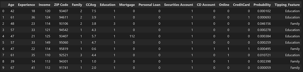
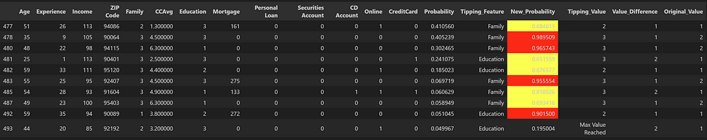
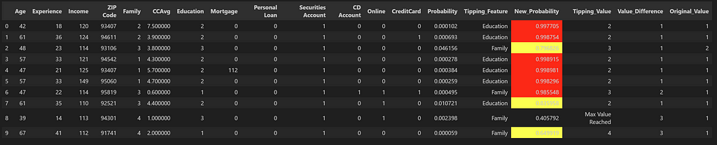
For evaluation, I have created a function which does a grid search on the values of Family or Education depending upon the Tipping_Feature for that customer from minimum value (which would be the current value) to the maximum value (which is the maximum value seen in the entire dataset for that feature) till the probability increases beyond 0.5.
List B Probabilities after changing the value for the Tipping_Feature
We see that with List B, the candidates which we got through the use of probabilities, there was one candidate which couldn’t move into the wanted category after changing the tipping_values. At the same time, there were 4 candidates (highlighted in red) which show very high probability of purchasing the loan after the tipping feature changes.
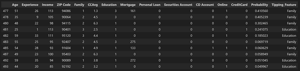
List A Probabilities after changing the value for the Tipping_Feature
For List A, we see that while there is one candidate which couldn’t tip over into the wanted category, there are 6 candidates (highlighted in red) which show very high probability once the tipping feature value is changed. We can also see that these candidates originally had very low probabilities of purchasing the loan and without the use of similarity search, these potential candidates would have been missed out.
Conclusion
While there can be other methods to search for potential candidates, similarity search using LLM vector embeddings can highlight candidates which would most likely not get prioritized otherwise. The method can have various usage and in this case was combined with the probabilities calculated with the help of XGBoost model.
Unless stated otherwise, all images are by the author.
We use cookies on our website to give you the most relevant experience by remembering your preferences and repeat visits. By clicking “Accept”, you consent to the use of ALL the cookies.
This website uses cookies to improve your experience while you navigate through the website. Out of these, the cookies that are categorized as necessary are stored on your browser as they are essential for the working of basic functionalities of the website. We also use third-party cookies that help us analyze and understand how you use this website. These cookies will be stored in your browser only with your consent. You also have the option to opt-out of these cookies. But opting out of some of these cookies may affect your browsing experience.
Necessary cookies are absolutely essential for the website to function properly. These cookies ensure basic functionalities and security features of the website, anonymously.
Cookie
Duration
Description
cookielawinfo-checkbox-analytics
11 months
This cookie is set by GDPR Cookie Consent plugin. The cookie is used to store the user consent for the cookies in the category "Analytics".
cookielawinfo-checkbox-functional
11 months
The cookie is set by GDPR cookie consent to record the user consent for the cookies in the category "Functional".
cookielawinfo-checkbox-necessary
11 months
This cookie is set by GDPR Cookie Consent plugin. The cookies is used to store the user consent for the cookies in the category "Necessary".
cookielawinfo-checkbox-others
11 months
This cookie is set by GDPR Cookie Consent plugin. The cookie is used to store the user consent for the cookies in the category "Other.
cookielawinfo-checkbox-performance
11 months
This cookie is set by GDPR Cookie Consent plugin. The cookie is used to store the user consent for the cookies in the category "Performance".
viewed_cookie_policy
11 months
The cookie is set by the GDPR Cookie Consent plugin and is used to store whether or not user has consented to the use of cookies. It does not store any personal data.
Functional cookies help to perform certain functionalities like sharing the content of the website on social media platforms, collect feedbacks, and other third-party features.
Performance cookies are used to understand and analyze the key performance indexes of the website which helps in delivering a better user experience for the visitors.
Analytical cookies are used to understand how visitors interact with the website. These cookies help provide information on metrics the number of visitors, bounce rate, traffic source, etc.
Advertisement cookies are used to provide visitors with relevant ads and marketing campaigns. These cookies track visitors across websites and collect information to provide customized ads.