Combine your React Application with the FastAPI web-server
In this guide, you will learn how to package a simple TypeScript React Application into a Python package and serve it from your FastAPI Python web server. Check out the client and the server repos, if you want to see the full code. Let’s get started!
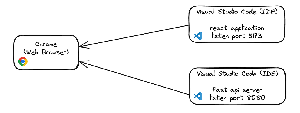
During the development process, you probably use two different IDEs:
TypeScript or JavaScript React App window, running on a dedicated listening port (e.g., 5173) to serve the client/frontend pages.
Python FastAPI, running on a different port (e.g., 8080) to serve a REST API.
In other words, you have two different servers running locally. Whenever you want to call your FastAPI server, the browser interacts with two different servers.
Local development (Image by Author)
While it works fine locally (in localhost), you’ll encounter a “Cross-Origin Request Blocked” error in your browser when you deploy that code. Before taking your code to production, the best practice is to serve both client pages and REST API from the same backend web server. That way the browser will interact with a single backend. It’s better for security, performance, and simplicity.
Preparing for Production (Image by Author)
1. Create a Simple React Application
First, in your workspace directory, let’s create a new TypeScript React application using vite:
At this point, the Backend Status is unknown because we haven’t implemented it yet. No worries, we will handle that shortly. Lastly, let’s build the client for packaging it later on:
~/workspace/vite-project ➜ npm run build
The build output should create a dist folder with the final optimized code that looks like this:
└── dist/
    ├── assets/
    ├── static/
    └── index.html
2. Building a Python Package
At this point, we are switching to Python. I prefer to work in a virtual environment for isolation. In a dedicated virtual environment, we will install twine and build , for creating our Python package:
Note that we installed our client package from a local path that we created earlier. If you uploaded your package to a remote repository, you can install it with:
Next, let’s create a simple Python server (2 files):
__main__.py
from distutils.sysconfig import get_python_lib from fastapi import FastAPI from fastapi.responses import FileResponse from fastapi.staticfiles import StaticFiles from backend.health_router import router from uvicorn import run
@router.get( "/liveness", summary="Perform a Liveness Health Check", response_description="Return HTTP Status Code 200 (OK)", status_code=status.HTTP_200_OK, response_model=ReturnHealthcheckStruct, ) async def liveness() -> ReturnHealthcheckStruct: return {"status": "success"}
In the implementation above, we added support for serving any static file from our client application by mounting the static and assets folders, as well as any other client file to be served by our Python server.
We also created a simple GET endpoint, v1/health-check/liveness that returns a simple {“status”: “success”} JSON response. That way we can ensure that our server handles both client static files and our server-side RESTful API.
Now, if we go to localhost:8080 we can see our client up and running. Pay attention to the Backend Status below, it’s now success (rather than unknown).
Running a Python server together with React Application (Image by Author)
Summary
In this tutorial, we created a simple React Application that does a single call to the backend. We wrapped this client application as a Python package and served it from our FastAPI Python web server.
Using this approach allows you to leverage the best tools in both worlds: TypeScript and React for the frontend, and Python with FastAPI for the backend. Yet, we want to keep high cohesion and low coupling between those two components. That way, you will get all the benefits:
Velocity, by separating front-end and backend to different repositories, each part can be developed by a different team.
Stability and Quality, by locking a versioned client package and bumping it only when the server is ready to support a new client version.
Safety — The browser interacts with only one backend server. We don’t need to enable CORS or any other security-compromising workarounds.
With a multitude of articles, videos, audio recordings, and other media created daily across news media companies, readers of all types—individual consumers, corporate subscribers, and more—often find it difficult to find news content that is most relevant to them. Delivering personalized news and experiences to readers can help solve this problem, and create more engaging […]
This is a guest post co-written with Tamir Rubinsky and Aviad Aranias from Nielsen Sports. Nielsen Sports shapes the world’s media and content as a global leader in audience insights, data, and analytics. Through our understanding of people and their behaviors across all channels and platforms, we empower our clients with independent and actionable intelligence […]
There’s always new and exciting terrain to discover in the field of geospatial data: from practical applications that help us better understand physical topography and social infrastructure, to theoretical approaches that allow us to navigate abstract spaces.
It’s been a while since we’ve covered this topic in the Variable, so this week we’re delighted to share a selection of recent articles that offer fascinating glimpses into work across the wide range of use cases that geospatial data encompasses. From beginner-friendly tutorials to more advanced theoretical questions, we’re certain you’ll find a lot here to pique your interest regardless of your background and level of experience.
Exploring Location Data Using a Hexagon Grid Leveraging the versatile data from Helsinki’s city bike program, Sara Tähtinen provides a detailed introduction to the power of Uber’s global H3 hexagonal grid system, which is both “a user-friendly and practical tool for spatial data analysis” and a handy method “to anonymize location data by aggregating geographic information to hexagonal regions.”
Depth Anything — A Foundation Model for Monocular Depth Estimation In a thoroughly explained paper walkthrough, Sascha Kirch unpacks the complexities of monocular depth estimation, “the prediction of distance in 3D space from a 2D image”—a problem that requires practitioners to apply their geospatial, computer vision, and deep learning skills, and that a new foundation model aims to solve.
Downscaling a Satellite Thermal Image from 1000m to 10m (Python) There are numerous ways to generate powerful environmental insights based on satellite images, but working with this type of data comes with its own set of challenges. Mahyar Aboutalebi, Ph.D. publishes frequently around this topic; one of his latest tutorials focuses on a Python-based approach for downscaling the thermal imagery captured by the Sentinel-2 and Sentinel-3 satellites.
How to Find Yourself in a Digital World Curious about the ever-evolving world of robotics? Eden B.’s debut TDS article zoomed in on the question of robots’ ability to self-localize, a crucial requirement for many common products (think: autonomous cars and delivery robots); their post goes on to outline how we can use probabilistic tools to compute localization.
Where Do EU Horizon H2020 Fundings Go? Geospatial analysis can be a useful first step on the path to answering questions that go far beyond geography. Case in point: Milan Janosov’s new tutorial, which brings together data analytics, network science, and a healthy dose of Python to map out thousands of EU-funded research and innovation projects.
Wait, there’s more! If you have the time to explore some other topics this week, here are some of our recent highlights:
Using VPython simulations to model chaotic motion and investigate what defines a chaotic system.
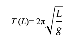
Any physics student has examined the lowly pendulum, probably more than they wanted to. Along with the mass on a spring, pendulums are the quintessential example of simple harmonic motion. The keyword there is simple. They, as you may know, are incredibly easy to model mathematically. The period of the pendulum can be represented by the formula below, where g is the force of gravity and L is the length of the pendulum.
The angular displacement is somewhat more interesting but still not too deep. The equation itself is more complex, but in reality it is just a cosine wave. The equation below represents the angular displacement of a single pendulum, where θ is the angular displacement, A is the maximum angular displacement (in most cases this is just the release angle), ω is the angular frequency, and t is time.
With that out of the way, let’s get to the more interesting, albeit effectively impossible (you’ll see), mathematics and physics.
Odds are, if you’ve worked with a regular pendulum, you’re at least somewhat familiar with the double pendulum, which is reminiscent of the infamous three-body problem. The three-body problem represents the idea that an analytical solution to the motion of three bodies in a system where all bodies’ forces affect each other is impossible to solve, since the forces of each body interact with the others simultaneously. In short, the double pendulum is impossible to solve analytically. In terms of the pendulum equations stated above, the one that you really can’t solve is the equation for θ, or the angular displacement of both pendulums. You also cannot solve for the period, but that’s mostly because a double pendulum doesn’t exactly have a regular period. Below is a visual representation of the double pendulum system we’ve discussed, where the pivot point is anchored to the wall, the angles are marked with θ1 and θ2, and the hanging masses are marked m1 and m2.
To reiterate– in our current physics, we cannot predict the motion of a double pendulum analytically. But why? Well, the motion is not simply random, but rather chaotic. How do we prove that chaotic and random aren’t the same? That is the question we will seek to answer later on.
You’ve likely seen some YouTube title about chaos or Chaos Theory, and I’m willing to bet the thumbnail image looked something like this:
That image, along with many other butterfly wing-esque drawings, are most commonly associated with chaos theory. Something not commonly thought of as part of chaos theory is the double, triple, and any other pendulum with more than one arm. Let’s explore some of the properties of chaotic motion and try to learn more about it as best we can, with help from a computer program that we will dive into later.
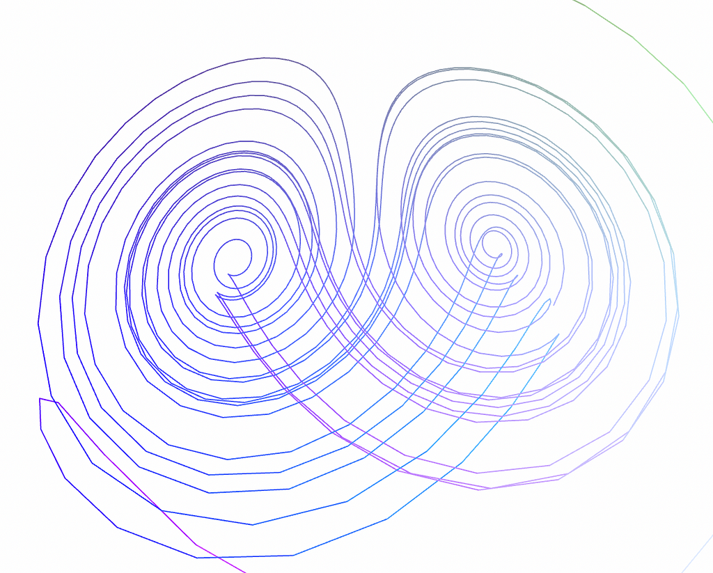
One property we can investigate is the effect that making a small change in starting conditions has on the end result. Will the change be negligible in the end, or will it yield an answer entirely outcome from the original?Below is a computer simulation of a double pendulum at t=50, where the starting angles were 80° and 0° respectively for θ1 and θ2. (Angles are the same as shown in the diagram above)
The red line drags behind the bottom mass (m2) of the pendulum, and remains for 2 seconds after being drawn.
Now, let’s run the exactsame simulation, the image is of t=50, all the masses and arm lengths are completely identical. However, the angles are 79° and 0° for θ1 and θ2. There’s a 1° change in the starting value of θ1, let’s see how it affects the outcome.
Unsurprisingly (or surprisingly, I don’t know what you expected), with a change of just 1° the system has dramatically changed to the point where the final position of the system and the line traced by it don’t resemble the first image at all. That’s independent of any outside variables, as in our simulation there is no friction, air resistance, or any other hindrances. This example shows the idea that when a system exhibits chaotic motion, as in a double pendulum, even the most minute change in conditions can cause an enormous change in the result.
So, we’ve nailed down one interesting aspect of chaotic motion– a tiny change in starting condition can cause an enormous change in result. Let’s try to identify a few more. What would happen if we were to run the same double pendulum experiment again? Experimentally, this is all but impossible; it would involve having an infinite degree of precision when measuring things like gravitational field, mass, air resistance, and every single other variable in the experiment, and then using your magical infinite precision data to set up the experiment again, identically. We, however, have a nice simulation to use which makes that challenge disappear.
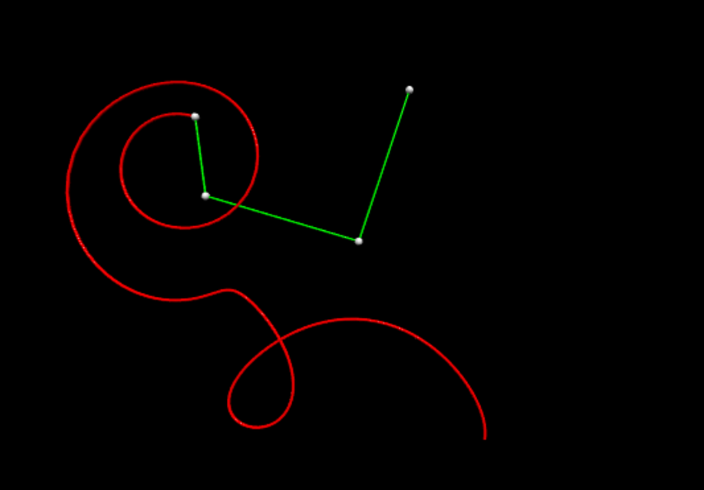
Let’s run the double pendulum simulation similar to before, but with some variables changed so the image isn’t the same: t=50, θ1=80°, θ2=15°, and the physical properties of the pendulum are the same (length, mass). Here is the result:
Spoiler alert, it was the exact same the second time… And the third, fourth fifth, and sixth time. Just to prove a point, let’s also try this exercise with a triple pendulum. We’ll use the same starting conditions, although now we have a third angle, θ3, so we’ll use θ1=80°, θ2=15°, θ3=0°. A triple pendulum is much more computationally intensive, though, so the image will be taken at t=10.
In the triple pendulum simulation, the red line is dragged behind the third mass.
Although it is even more complex than the double pendulum simulation, the fact that the triple pendulum exhibits the same tendency to repeat its pattern under identical starting conditions is important. That idea of an identical outcome under identical conditions proves that chaotic motion and chaotic systems are deterministic, thus not random. Again, since this is so hard to prove experimentally or use in practice it doesn’t affect our understanding of the real world very much. We do, however, now know that chaotic systems are not random and can be predicted with the right knowledge. Additionally, since we proved that a small change can have a large effect, we know that an incredibly high degree of precision is needed to effectively predict the outcome of a chaotic system.
We’ve now identified two significant properties of chaotic motion: the first is that a tiny change can have huge implications in the outcome of the system, and the second is that chaotic motion is not random but rather it is deterministic. Let’s try to fine one more– as we discussed at the very beginning of the article, the variable you really can’t solve for in a double pendulum is the angular displacement. However, we also said that solving for period was futile because a double pendulum does not repeat– let’s test that theory.
First, let’s run the double pendulum experiment with the following conditions: θ1=30°, θ2=30°, with the same masses and lengths as before. This time, let’s use VPython’s graphing capabilities to record a chart of the height of the bottom mass as a function of time:
If you ask me, that looks pretty periodic. So, does this mean that the system described above is not a chaotic system? And if the motion is not chaotic, does that mean we could reach an analytical solution to the motion of the double pendulum when it has less than some threshold energy needed to become chaotic? I’ll leave that as an exercise to the reader. To do that though, you might need the help of the program I wrote and used in this article, so let’s walk through it. This program is written in VPython using GlowScript, so be sure that you’re running it on the WebVPython system, and not just any python editor.
First, let’s define the physical constants we’ll use in the program. These include the masses, lengths of arms, and force of gravity. Additionally, we’ll define the starting conditions of the system, where theta1 and theta2 are the starting angles, and theta1dot and theta2dot are the starting angular velocities of the arms. Finally we’ll also set the starting time to 0, and define dt, which is the amount of time we’ll step forwards in each iteration of our loop later.
#lengths of the strings L1 = 1.5 #top string L2 = 1 #middle string
Next we define all the parts of our system, the pivot point, mass 1 (m1), arm 1 (stick1), and the same for the second set of mass and stick (m2, stick2).
Now we position the masses and sticks so that they reflect the starting angles, as if you ran the code before it would just be two vertical rods. To do this we just use some trigonometry to put the mass the end of where the stick will go, then set the stick to go the distance between each mass. Here we also use VPython’s ‘attach_trail’ method to make the bottom mass generate a trail.
Next we begin the main loop of our program; in this simulation, as in many physics simulations we’ll use a while loop with an exit condition at t=50. We’ll also use the the rate() method to set the speed that the program will run at.
while t <= 50:
    rate(1000)
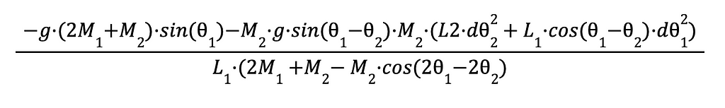
Now we have to dive into the real math. We’ll use a bit of calculus (not really, but we do deal with derivatives), trigonometry, and algebra to first calculate the angular acceleration, which we will then use to increment the angular velocity, and then apply that angular velocity to the position of the masses and rods to move them according to their calculated accelerations.
To calculate the top mass’s acceleration, let’s use this formula to represent the angular acceleration, or second derivative of θ1:
You can also represent the same equation using the following code:
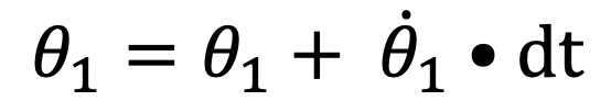
Next let’s increment the variables for angular velocity, ‘theta1dot’ and ‘theta2dot.’ To do this we simply use the equation below, which increments the angular velocity by the angular acceleration times dt. Although the image only states the equation for theta1dot, it is the same for both θ1 and θ2.
For the final part of our calculations for the motion of the double pendulum must increment the angles θ1 and θ2 by the angular velocity. This is represented by the equation below, where we set the angle θ equal to the previous θ plus the angular velocity times dt. Again, the calculation is the exact same for θ1 and θ2.
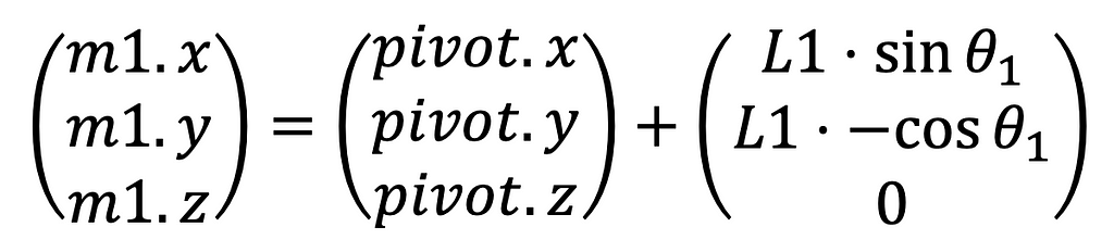
Now we must update the position of the masses and the rods in the program, so that we can see the outcome of the program. First we will update the position of the masses. We’ll take an intuitive approach to updating these positions; since one thing that will never change in the system is the length of the rods, the middle mass (m1) will be a distance equal to L1 away from the pivot point. Logically we can then construct the following equation for the position of mass m1:
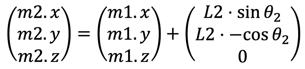
The same formula can be used to reflect the formula for the position of m2, only with θ2 and L2, and it is based off of the position of m1, not the pivot. See this equation below.
These two formulas are written in our program very simply, since one feature of VPython is that it makes vector calculations very simple. All objects already have their positions stored as vectors, so all you need to do is use the vector() method to define a new vector, and use it in your computation.
Now we must take one final step to realize the outcome of our calculations by updating the position of the rods. Technically this isn’t totally necessary, as the masses will still show and follow the pattern they should. For visual effect though, let’s write this code. The math isn’t too interesting, so the code is as follows. First we set the axis of the first stick so that it fills the distance between the pivot point and mass m1. Next, we set the second stick’s position equal to mass m1. Finally, we set the axis of the second stick equal to the distance between the first and second mass. The final line is incrementing t by dt to make the program go forwards.
Thank you for making it this far, I hope you enjoyed my analysis of chaotic motion through the double and triple pendulums. In the end, I’m neither a professional physicist nor programmer, so if you have suggestions for how I can improve my work please don’t hesitate to let me know.
Additionally, all imaged used in the article were created by me, using Python and Microsoft Word, both of which have incredible capabilities.
Finally, I’d like to end on a chewy thought, which will play into my next project. If you took a multi-armed pendulum which was already experiencing chaotic motion, how would its motion change if you were to seamlessly add another arm of very high mass (maybe 50x the largest already in a system), at a starting θ of 0°?
We use cookies on our website to give you the most relevant experience by remembering your preferences and repeat visits. By clicking “Accept”, you consent to the use of ALL the cookies.
This website uses cookies to improve your experience while you navigate through the website. Out of these, the cookies that are categorized as necessary are stored on your browser as they are essential for the working of basic functionalities of the website. We also use third-party cookies that help us analyze and understand how you use this website. These cookies will be stored in your browser only with your consent. You also have the option to opt-out of these cookies. But opting out of some of these cookies may affect your browsing experience.
Necessary cookies are absolutely essential for the website to function properly. These cookies ensure basic functionalities and security features of the website, anonymously.
Cookie
Duration
Description
cookielawinfo-checkbox-analytics
11 months
This cookie is set by GDPR Cookie Consent plugin. The cookie is used to store the user consent for the cookies in the category "Analytics".
cookielawinfo-checkbox-functional
11 months
The cookie is set by GDPR cookie consent to record the user consent for the cookies in the category "Functional".
cookielawinfo-checkbox-necessary
11 months
This cookie is set by GDPR Cookie Consent plugin. The cookies is used to store the user consent for the cookies in the category "Necessary".
cookielawinfo-checkbox-others
11 months
This cookie is set by GDPR Cookie Consent plugin. The cookie is used to store the user consent for the cookies in the category "Other.
cookielawinfo-checkbox-performance
11 months
This cookie is set by GDPR Cookie Consent plugin. The cookie is used to store the user consent for the cookies in the category "Performance".
viewed_cookie_policy
11 months
The cookie is set by the GDPR Cookie Consent plugin and is used to store whether or not user has consented to the use of cookies. It does not store any personal data.
Functional cookies help to perform certain functionalities like sharing the content of the website on social media platforms, collect feedbacks, and other third-party features.
Performance cookies are used to understand and analyze the key performance indexes of the website which helps in delivering a better user experience for the visitors.
Analytical cookies are used to understand how visitors interact with the website. These cookies help provide information on metrics the number of visitors, bounce rate, traffic source, etc.
Advertisement cookies are used to provide visitors with relevant ads and marketing campaigns. These cookies track visitors across websites and collect information to provide customized ads.