Structured Query Language (SQL) is an essential tool for data professionals such as data scientists and data analysts as it allows them to retrieve, manipulate, and analyze large datasets efficiently and effectively. It is a widely used tool in the industry, making it an important skill to have. In this article, I want to share how to create Pivot tables in SQL. This article follows up on my last article “Pandas!!! What I’ve Learned after my 1st On-site Technical Interview”, where I shared my learnings on Pandas.
Did you know that SQL can be used to analyze data?
In SQL, a Pivot table is a technique used to transform data from rows to columns.
Joan Casteel’s Oracle 12c: SQL book mentions that “a pivot table is a presentation of multidimensional data.” With a pivot table, a user can view different aggregations of different data dimensions. It is a powerful tool for data analysis, as it allows users to aggregate, summarize, and present data in a more intuitive and easy-to-read format.
For instance, an owner of an ice cream shop may want to analyze which flavor of ice cream has sold the best in the past week. A pivot table would be useful in this case, with two dimensions of data — ice cream flavor and day of the week. Revenue can be summed up as the aggregation for the analysis.
The ice cream shop owner can easily use a pivot table to compare sales by ice cream flavor and day of the week. The pivot table will transform the data, making it easier to spot patterns and trends. With this information, the owner can make data-driven decisions, such as increasing the supply of the most popular ice cream flavor or adjusting the prices based on demand.
Overall, pivot tables are an excellent tool for data analysis, allowing users to summarize and present multidimensional data in a more intuitive and meaningful way. They are widely used in industries such as finance, retail, and healthcare, where there is a need to analyze large amounts of complex data.
This article will be based on the analytic function in Oracle, typically the “PIVOT” function. It is organized to provide a comprehensive view of utilizing pivot tables in SQL in different situations. We will not only go through the most naive way to create a pivot table but also the easiest and most common way to do the job with the PIVOT function. Last but not least, I will also talk about some of the limitations of the PIVOT function.
FYI:
I will use Oracle 11g, but the functions are the same in the newer Oracle 12c and above.
The demonstration dataset is Microsoft’s Northwind dataset. The sales data for Northwind Traders, a fictitious specialty foods export/import company. The database is free of use and widely distributed for learning and demonstration purposes. Be sure to set up the database environment beforehand! I also attached the Northwind schema below:
The crudest way to pivot a table is to utilize the function: DECODE(). DECODE() function is like an if else statement. It compares the input with each value and produces an output.
input/value: “input” is compared with all the “values”.
return: if input = value, then “return” is the output.
default (optional): if input != all of the values, then “default” is the output.
When we know how DECODE() works, it is time to make our first pivot table.
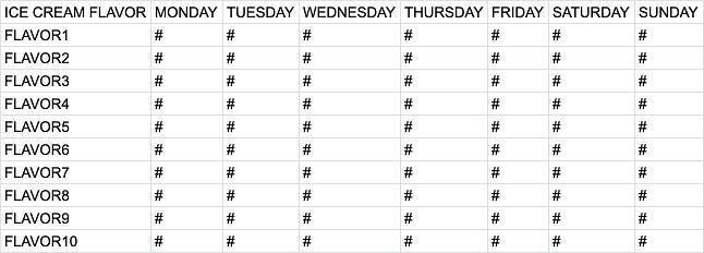
1st Version: Pivot table without total column and row
Pivot table without total column and row, Source: Me
With DECODE(), we can map out a pseudocode of a pivot table for the ice cream shop owner. When the “day of the week” matches each weekday, DECODE() returns the day’s revenue; if it does not match, 0 is returned instead.
SELECT ice cream flavor,
SUM(DECODE(day of the week, 'Monday', revenue, 0)) AS MONDAY, SUM(DECODE(day of the week, 'Tuesday', revenue, 0)) AS TUESDAY,
SUM(DECODE(day of the week, 'Wednesday', revenue, 0)) AS WEDNESDAY,
SUM(DECODE(day of the week, 'Thursday', revenue, 0)) AS THURSDAY,
SUM(DECODE(day of the week, 'Friday', revenue, 0)) AS FRIDAY,
SUM(DECODE(day of the week, 'Saturday', revenue, 0)) AS SATURDAY,
SUM(DECODE(day of the week, 'Sunday', revenue, 0)) AS SUNDAY
FROM ice cream shop dataset
WHERE date between last Monday and last Sunday;
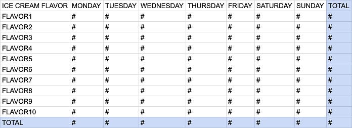
2nd Version: Pivot table with total column and row
Pivot table with total column and row, Source: Me
Great job! Now the ice cream shop owner wants to know more about what happened with last week’s sales. You could upgrade your pivot table by adding a total column and total row.
This could be accomplished using the GROUPING SETS Expression in a GROUP BY statement. A GROUPING SETS Expression defines criteria for multiple GROUP BY aggregations.
GROUPING SETS (attribute1, …, ())
attribute: a single element or a list of elements to GROUP BY
(): an empty group, which will become the pivot table’s TOTAL row
SELECT NVL(ice cream flavor, 'TOTAL') "ICE CREAM FLAVOR",
SUM(DECODE(day of the week, 'Monday', revenue, 0)) AS MONDAY, SUM(DECODE(day of the week, 'Tuesday', revenue, 0)) AS TUESDAY,
SUM(DECODE(day of the week, 'Wednesday', revenue, 0)) AS WEDNESDAY,
SUM(DECODE(day of the week, 'Thursday', revenue, 0)) AS THURSDAY,
SUM(DECODE(day of the week, 'Friday', revenue, 0)) AS FRIDAY,
SUM(DECODE(day of the week, 'Saturday', revenue, 0)) AS SATURDAY,
SUM(DECODE(day of the week, 'Sunday', revenue, 0)) AS SUNDAY,
SUM(revenue) AS TOTAL
FROM ice cream shop dataset
WHERE date between last Monday and last Sunday
GROUP BY GROUPING SETS (ice cream flavor, ());
Note: NVL() replaces the null row created by () with ‘TOTAL.’ If you are unfamiliar with NVL(), it is simply a function to replace null values.
Another way of calculating the TOTAL column is to add all the revenue from MONDAY to SUNDAY:
SUM(DECODE(day of the week, 'Monday', revenue, 0))
+ SUM(DECODE(day of the week, 'Tuesday', revenue, 0))
+ SUM(DECODE(day of the week, 'Wednesday', revenue, 0))
+ SUM(DECODE(day of the week, 'Thursday', revenue, 0))
+ SUM(DECODE(day of the week, 'Friday', revenue, 0))
+ SUM(DECODE(day of the week, 'Saturday', revenue, 0))
+ SUM(DECODE(day of the week, 'Sunday', revenue, 0)) AS TOTAL
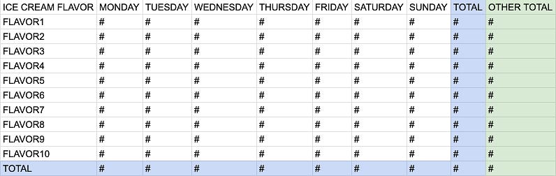
3rd Version: Pivot table with total column and row and other totals
Pivot table with total column and row and other totals, Source: Me
Say that the ice cream owner wanted one more column on the pivot table you provided: the total number of purchases of each flavor of ice cream. No problem! You can add another “TOTAL” column with the same concept!
SELECT NVL(ice cream flavor, 'TOTAL') "ICE CREAM FLAVOR",
SUM(DECODE(day of the week, 'Monday', revenue, 0)) AS MONDAY, SUM(DECODE(day of the week, 'Tuesday', revenue, 0)) AS TUESDAY,
SUM(DECODE(day of the week, 'Wednesday', revenue, 0)) AS WEDNESDAY,
SUM(DECODE(day of the week, 'Thursday', revenue, 0)) AS THURSDAY,
SUM(DECODE(day of the week, 'Friday', revenue, 0)) AS FRIDAY,
SUM(DECODE(day of the week, 'Saturday', revenue, 0)) AS SATURDAY,
SUM(DECODE(day of the week, 'Sunday', revenue, 0)) AS SUNDAY,
SUM(revenue) AS TOTAL,
SUM(purchase ID) "OTHER TOTAL"
FROM ice cream shop dataset
WHERE date between last Monday and last Sunday
GROUP BY GROUPING SETS (ice cream flavor, ());
Now that you know how to do a pivot table with DECODE(), let’s try three exercises with the Northwind dataset!
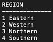
Q1. Let’s say we want to find out how many employees in each of their origin countries serve in each region.
To break up this question, first, we can query all distinct regions in the REGION table. Also, check what countries the employees are from.
SELECT DISTINCT REGIONID||' '||RDescription AS REGION
FROM REGION
ORDER BY 1;
SELECT DISTINCT Country
FROM EMPLOYEES
ORDER BY 1;
We will have to make a 2 * 4 pivot table for this question.
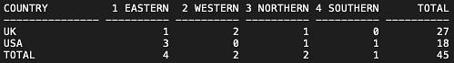
Next, we can make a pivot table using DECODE(). A sample answer and output are outlined below:
SELECT NVL(Country, 'TOTAL') AS COUNTRY,
SUM(DECODE(LOWER(REGIONID||' '||RDescription), '1 eastern', 1, 0)) "1 EASTERN",
SUM(DECODE(LOWER(REGIONID||' '||RDescription), '2 western', 1, 0)) "2 WESTERN",
SUM(DECODE(LOWER(REGIONID||' '||RDescription), '3 northern', 1, 0)) "3 NORTHERN",
SUM(DECODE(LOWER(REGIONID||' '||RDescription), '4 southern', 1, 0)) "4 SOUTHERN",
SUM(EmployeeID) AS TOTAL
FROM EMPLOYEES
JOIN REGION USING (REGIONID)
GROUP BY GROUPING SETS (Country, ());
--Q1
SELECT Country,
SUM(DECODE(LOWER(REGIONID||' '||RDescription), '1 eastern', 1, 0)) "1 EASTERN",
SUM(DECODE(LOWER(REGIONID||' '||RDescription), '2 western', 1, 0)) "2 WESTERN",
SUM(DECODE(LOWER(REGIONID||' '||RDescription), '3 northern', 1, 0)) "3 NORTHERN",
SUM(DECODE(LOWER(REGIONID||' '||RDescription), '4 southern', 1, 0)) "4 SOUTHERN",
SUM() AS TOTAL
FROM EMPLOYEES
JOIN REGION USING (REGIONID)
GROUP BY Country;
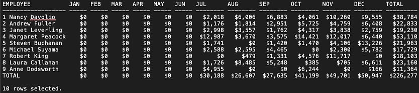
Q2. For each month in 2010, show the revenue of orders processed by each employee. Also, round to the nearest dollar and display the total revenue made and the total number of orders.
--Q2
COLUMN EMPLOYEE FORMAT A18
SELECT NVL(EmployeeID||' '||FirstName||' '||LastName, 'TOTAL') AS EMPLOYEE,
TO_CHAR(SUM(DECODE(EXTRACT(MONTH FROM OrderDate), 1, (UnitPrice * Quantity - Discount), 0)), '$990') AS JAN,
TO_CHAR(SUM(DECODE(EXTRACT(MONTH FROM OrderDate), 2, (UnitPrice * Quantity - Discount), 0)), '$990') AS FEB,
TO_CHAR(SUM(DECODE(EXTRACT(MONTH FROM OrderDate), 3, (UnitPrice * Quantity - Discount), 0)), '$990') AS MAR,
TO_CHAR(SUM(DECODE(EXTRACT(MONTH FROM OrderDate), 4, (UnitPrice * Quantity - Discount), 0)), '$990') AS APR,
TO_CHAR(SUM(DECODE(EXTRACT(MONTH FROM OrderDate), 5, (UnitPrice * Quantity - Discount), 0)), '$990') AS MAY,
TO_CHAR(SUM(DECODE(EXTRACT(MONTH FROM OrderDate), 6, (UnitPrice * Quantity - Discount), 0)), '$990') AS JUN,
TO_CHAR(SUM(DECODE(EXTRACT(MONTH FROM OrderDate), 7, (UnitPrice * Quantity - Discount), 0)), '$99,990') AS JUL,
TO_CHAR(SUM(DECODE(EXTRACT(MONTH FROM OrderDate), 8, (UnitPrice * Quantity - Discount), 0)), '$99,990') AS AUG,
TO_CHAR(SUM(DECODE(EXTRACT(MONTH FROM OrderDate), 9, (UnitPrice * Quantity - Discount), 0)), '$99,990') AS SEP,
TO_CHAR(SUM(DECODE(EXTRACT(MONTH FROM OrderDate), 10, (UnitPrice * Quantity - Discount), 0)), '$99,990') AS OCT,
TO_CHAR(SUM(DECODE(EXTRACT(MONTH FROM OrderDate), 11, (UnitPrice * Quantity - Discount), 0)), '$99,990') AS NOV,
TO_CHAR(SUM(DECODE(EXTRACT(MONTH FROM OrderDate), 12, (UnitPrice * Quantity - Discount), 0)), '$99,990') AS DEC,
TO_CHAR(SUM((UnitPrice * Quantity - Discount)), '$999,990') AS TOTAL
FROM ORDERS
JOIN ORDERDETAILS USING (OrderID)
JOIN EMPLOYEES USING (EmployeeID)
WHERE EXTRACT(YEAR FROM OrderDate) = 2010
GROUP BY GROUPING SETS (EmployeeID||' '||FirstName||' '||LastName, ())
ORDER BY 1;
Note: Notice the FORMAT command and TO_CHAR() function are for formatting purposes. If you want to learn more, please check out the Format Models and Formatting SQL*Plus Reports section on Oracle’s website.
Now that you know how to make a pivot table with DECODE(), we can move on to the PIVOT() clause introduced to Oracle in its 11g version.
SELECT * FROM ( query) PIVOT (aggr FOR column IN (value1, value2, …) );
aggr: function such as SUM, COUNT, MIN, MAX, or AVG
value: A list of values for column to pivot into headings in the cross-tabulation query results
Let’s get back to the ice cream shop example. Here is how we can make it with the PIVOT() clause:
1st Version: Pivot table without total column and row
SELECT *
FROM (
      SELECT day of the week, ice cream flavor, revenue
      FROM ice cream shop dataset
      WHERE date between last Monday and last Sunday
)
PIVOT (
       SUM(revenue)
       FOR day of the week IN ('Monday', 'Tuesday', 'Wednesday', 'Thursday', 'Friday', 'Saturday', 'Sunday')
);
2nd Version: Pivot table with total column and row
If you want to add a total column to your pivot table, doing it with the NVL() function is a great way.
SELECT *
FROM (
      SELECT NVL(ice cream flavor, 'TOTAL') AS ice cream flavor,
             NVL(day of the week, -1) AS DOW,
             SUM(revenue) AS REV
      FROM ice cream shop dataset
      WHERE date between last Monday and last Sunday
      GROUP BY CUBE (ice cream flavor, day of the week)
)
PIVOT (
       SUM(REV)
       FOR DOW IN ('Monday', 'Tuesday', 'Wednesday', 'Thursday', 'Friday', 'Saturday', 'Sunday', -1 AS TOTAL)
);
3rd Version: Pivot table with total column and row and other totals
When other totals come into the scene, there is only one way to solve the problem. That is by using the JOIN() clause:
SELECT ice cream flavor, Monday, Tuesday, Wednesday, Thursday, Friday, Saturday, Sunday, TOTAL, OTHER TOTAL
FROM (
      SELECT NVL(ice cream flavor, 'TOTAL') AS ice cream flavor,
             NVL(day of the week, -1) AS DOW,
             SUM(revenue) AS REV
      FROM ice cream shop dataset
      WHERE date between last Monday and last Sunday
      GROUP BY CUBE (ice cream flavor, day of the week)
)
PIVOT (
       SUM(REV)
       FOR DOW IN ('Monday', 'Tuesday', 'Wednesday', 'Thursday', 'Friday', 'Saturday', 'Sunday', -1 AS TOTAL)
)
JOIN (
      SELECT NVL(ice cream flavor, 'TOTAL') AS ice cream flavor,
             SUM(purchase ID) "OTHER TOTAL"
      FROM ice cream shop dataset
      WHERE date between last Monday and last Sunday
      GROUP BY ROLLUP (ice cream flavor)
) USING (ice cream flavor);
Note: In the pseudocode above, We utilize the CUBE and ROLLUP Extension in GROUP BY. A small explanation will do the job.
Once we know how the PIVOT() clause work, can you practice it with the Northwind dataset we have in part 1?
Q1. Let’s say we want to find out how many employees in each of their origin countries serve in each region.
--Q1
--Try it out!
Q2. For each month in 2010, show the revenue of orders processed by each employee. Also, round to the nearest dollar and display the total revenue made and the total number of orders.
--Q2
--Try it out!
Epilogue
In this guide, we’ve explored the powerful capabilities of pivot tables in SQL, focusing on both the DECODE() and PIVOT() functions. We began with an introduction to pivot tables and their significance in transforming rows into columns for enhanced data analysis. We then walked through the process of creating pivot tables using DECODE() and examined the more streamlined PIVOT() function introduced in Oracle 11g, which simplifies pivot table creation. By applying these techniques, we’ve demonstrated how to efficiently analyze multidimensional data with practical examples, such as the ice cream shop dataset.
Pivot tables with DECODE(): A fundamental approach using the DECODE() function to manually pivot data.
Pivot tables with PIVOT(): Utilizing the PIVOT() function for a more efficient and readable pivot table creation.
Feel free to share your answers in the comments. I love to learn about data and reflect on (write about) what I’ve learned in practical applications. If you enjoyed this article, please give it a clap to show your support. You can contact me via LinkedIn and Twitter if you have more to discuss. Also, feel free to follow me on Medium for more data science articles to come!
A new alternative to the classic Multi-Layer Perceptron is out. Why is it more accurate and interpretable? Math and Code Deep Dive.
Image generated by DALL-E
In today’s world of AI, neural networks drive countless innovations and advancements. At the heart of many breakthroughs is the Multi-Layer Perceptron (MLP), a type of neural network known for its ability to approximate complex functions. But as we push the boundaries of what AI can achieve, we must ask: Can we do better than the classic MLP?
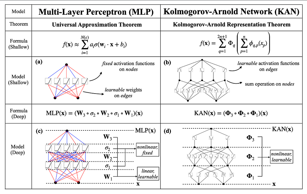
Here’s Kolmogorov-Arnold Networks (KANs), a new approach to neural networks inspired by the Kolmogorov-Arnold representation theorem. Unlike traditional MLPs, which use fixed activation functions at each neuron, KANs use learnable activation functions on the edges (weights) of the network. This simple shift opens up new possibilities in accuracy, interpretability, and efficiency.
This article explores why KANs are a revolutionary advancement in neural network design. We’ll dive into their mathematical foundations, highlight the key differences from MLPs, and show how KANs can outperform traditional methods.
1: Limitations of MLPs
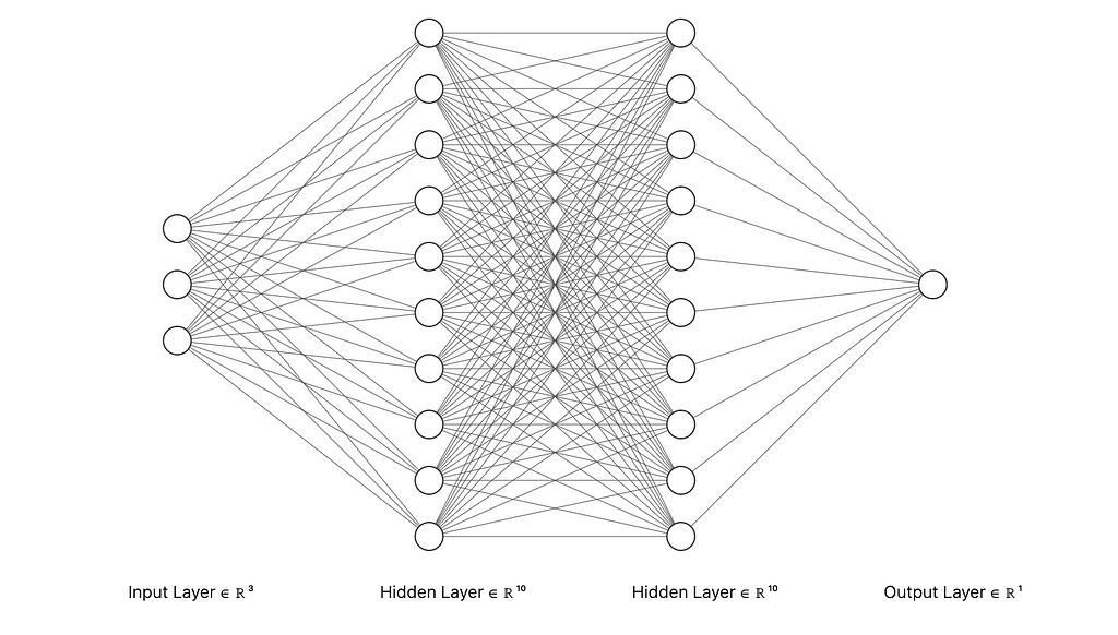
MLP with input layer with 3 nodes, 2 hidden layers with 10 nodes each, and an output layer with 1 node — Image by Author
Multi-Layer Perceptrons (MLPs) are a core component of modern neural networks. They consist of layers of interconnected nodes, or “neurons,” designed to approximate complex, non-linear functions by learning from data. Each neuron uses a fixed activation function on the weighted sum of its inputs, transforming input data into the desired output through multiple layers of abstraction. MLPs have driven breakthroughs in various fields, from computer vision to speech recognition.
However, MLPs have some significant limitations:
Fixed Activation Functions on Nodes: Each node in an MLP has a predetermined activation function, like ReLU or Sigmoid. While effective in many cases, these fixed functions limit the network’s flexibility and adaptability. This can make it challenging for MLPs to optimize certain types of functions or adapt to specific data characteristics.
Interpretability Issues: MLPs are often criticized for being “black boxes.” As they become more complex, understanding their decision-making process becomes harder. The fixed activation functions and intricate weight matrices obscure the network’s inner workings, making it difficult to interpret and trust the model’s predictions without extensive analysis.
These drawbacks highlight the need for alternatives that offer greater flexibility and interpretability, paving the way for innovations like Kolmogorov-Arnold Networks (KANs).
The Kolmogorov-Arnold representation theorem, formulated by mathematicians Andrey Kolmogorov and Vladimir Arnold, states that any multivariate continuous function can be represented as a finite composition of continuous functions of a single variable and the operation of addition. Think of this theorem as breaking down a complex recipe into individual, simple steps that anyone can follow. Instead of dealing with the entire recipe at once, you handle each step separately, making the overall process more manageable. This theorem implies that complex, high-dimensional functions can be broken down into simpler, univariate functions.
For neural networks, this insight is revolutionary, it suggests that a network could be designed to learn these univariate functions and their compositions, potentially improving both accuracy and interpretability.
KANs leverage the power of the Kolmogorov-Arnold theorem by fundamentally altering the structure of neural networks. Unlike traditional MLPs, where fixed activation functions are applied at each node, KANs place learnable activation functions on the edges (weights) of the network. This key difference means that instead of having a static set of activation functions, KANs adaptively learn the best functions to apply during training. Each edge in a KAN represents a univariate function parameterized as a spline, allowing for dynamic and fine-grained adjustments based on the data.
This change enhances the network’s flexibility and ability to capture complex patterns in data, providing a more interpretable and powerful alternative to traditional MLPs. By focusing on learnable activation functions on edges, KANs effectively utilize the Kolmogorov-Arnold theorem to transform neural network design, leading to improved performance in various AI tasks.
3: Mathematical Foundations
At the core of Kolmogorov-Arnold Networks (KANs) is a set of equations that define how these networks process and transform input data. The foundation of KANs lies in the Kolmogorov-Arnold representation theorem, which inspires the structure and learning process of the network.
Imagine you have an input vector x=[x1,x2,…,xn], which represents data points that you want to process. Think of this input vector as a list of ingredients for a recipe.
The theorem states that any complex recipe (high-dimensional function) can be broken down into simpler steps (univariate functions). For KANs, each ingredient (input value) is transformed through a series of simple steps (univariate functions) placed on the edges of the network. Mathematically, this can be represented as:
KAN Formula — Image by Author
Here, ϕ_q,p are univariate functions that are learned during training. Think of ϕ_q,p as individual cooking techniques for each ingredient, and Φ_q as the final assembly step that combines these prepared ingredients.
Each layer of a KAN applies these cooking techniques to transform the ingredients further. For layer l, the transformation is given by:
Kan Layer Transformation Formula — Image by Author
Here, x(l) denotes the transformed ingredients at layer l, and ϕ_l,i,j are the learnable univariate functions on the edges between layer l and l+1. Think of this as applying different cooking techniques to the ingredients at each step to get intermediate dishes.
The output of a KAN is a composition of these layer transformations. Just as you would combine intermediate dishes to create a final meal, KANs combine the transformations to produce the final output:
KAN Output Formula — Image by Author
Here, Φl represents the matrix of univariate functions at layer l. The overall function of the KAN is a composition of these layers, each refining the transformation further.
MLPs Structure In traditional MLPs, each node applies a fixed activation function (like ReLU or sigmoid) to its inputs. Think of this as using the same cooking technique for all ingredients, regardless of their nature.
MLPs use linear transformations followed by these fixed non-linear activations:
MLP Formula — Image by Author
where W represents the weight matrices, and σ represents the fixed activation functions.
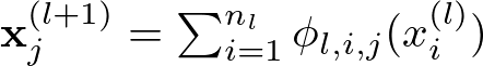
Grid Extension Technique
Left: Notations of activations that flow through the network. Right: an activation function is parameterized as a B-spline, which allows switching between coarse-grained and fine-grained grids — Imagine extracted by “KAN: Kolmogorov-Arnold Networks” (License)
Grid extension is a powerful technique used to improve the accuracy of Kolmogorov-Arnold Networks (KANs) by refining the spline grids on which the univariate functions are defined. This process allows the network to learn increasingly detailed patterns in the data without requiring complete retraining.
These B-splines are a series of polynomial functions that are pieced together to form a smooth curve. They are used in KANs to represent the univariate functions on the edges. The spline is defined over a series of intervals called grid points. The more grid points there are, the finer the detail that the spline can capture
Initially, the network starts with a coarse grid, which means there are fewer intervals between grid points. This allows the network to learn the basic structure of the data without getting bogged down in details. Think of this like sketching a rough outline before filling in the fine details.
As training progresses, the number of grid points is gradually increased. This process is known as grid refinement. By adding more grid points, the spline becomes more detailed and can capture finer patterns in the data. This is similar to progressively adding more detail to your initial sketch, turning it into a detailed drawing.
Each increase introduces new B-spline basis functions B′_m(x). The coefficients c’_m for these new basis functions are adjusted to ensure that the new, finer spline closely matches the original, coarser spline.
To achieve this match, least squares optimization is used. This method adjusts the coefficients c’_m to minimize the difference between the original spline and the refined spline.
Least Square Optimization Formula — Image by Author
Essentially, this process ensures that the refined spline continues to accurately represent the data patterns learned by the coarse spline.
Simplification Techniques
To enhance the interpretability of KANs, several simplification techniques can be employed, making the network easier to understand and visualize.
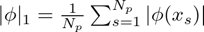
Sparsification and Pruning This technique involves adding a penalty to the loss function based on the L1 norm of the activation functions. The L1 norm for a function ϕ is defined as the average magnitude of the function across all input samples:
L1 Norm Formula — Image by Author
Here, N_p is the number of input samples, and ϕ(x_s) represents the value of the function ϕ for the input sample x_s.
Think of sparsification like decluttering a room. By removing unnecessary items (or reducing the influence of less important functions), you make the space (or network) more organized and easier to navigate.
After applying L1 regularization, the L1 norms of the activation functions are evaluated. Neurons and edges with norms below a certain threshold are considered insignificant and are pruned away. The threshold for pruning is a hyperparameter that determines how aggressive the pruning should be.
Pruning is like trimming a tree. By cutting away the weak and unnecessary branches, you allow the tree to focus its resources on the stronger, more vital parts, leading to a healthier and more manageable structure.
Symbolification Another approach is to replace learned univariate functions with known symbolic forms to make the network more interpretable.
The task is to identify potential symbolic forms (e.g., sin, exp) that can approximate the learned functions. This step involves analyzing the learned functions and suggesting symbolic candidates based on their shape and behavior.
Once symbolic candidates are identified, use grid search and linear regression to fit parameters such that the symbolic function closely approximates the learned function.
4: KAN vs MLP in Python
To demonstrate the capabilities of Kolmogorov-Arnold Networks (KANs) compared to traditional Multi-Layer Perceptrons (MLPs), we will fit a function-generated dataset to both a KAN model and MLP model (leveraging PyTorch), to see what their performances look like.
The function we will be using is the same one used by the authors of the paper to show KAN’s capabilities vs MLP (Original paper example). However, the code will be different. You can find all the code we will cover today in this Notebook:
Let’s import the required libraries, and generate the dataset
import numpy as np
import torch
import torch.nn as nn
from torchsummary import summary
from kan import KAN, create_dataset
import matplotlib.pyplot as plt
Here, we use:
numpy: For numerical operations.
torch: For PyTorch, which is used for building and training neural networks.
torch.nn: For neural network modules in PyTorch.
torchsummary: For summarizing the model structure.
kan: Custom library containing the KAN model and dataset creation functions.
matplotlib.pyplot: For plotting and visualizations.
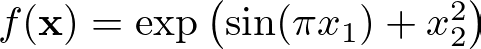
# Define the dataset generation function
f = lambda x: torch.exp(torch.sin(torch.pi * x[:, [0]]) + x[:, [1]] ** 2)
This function includes both sinusoidal (sin) and exponential (exp) components. It takes a 2D input x and computes the output using the formula:
Dataset generation Function — Image by Author
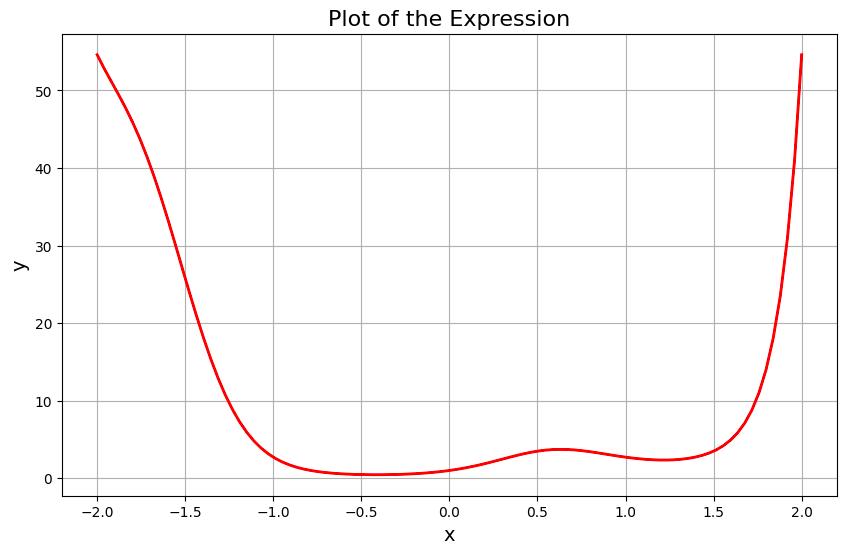
Let’s now fit a tensor of 100 points uniformly distributed between [-2, 2] to this function, to see what it looks like:
Plot generated by fitting 100 points uniformly distributed between [-2, 2] to Dataset generation function — Image by Author
# Create the dataset
dataset = create_dataset(f, n_var=2)
create_dataset generates a dataset based on the function f. The dataset includes input-output pairs that will be used for training and testing the neural networks.
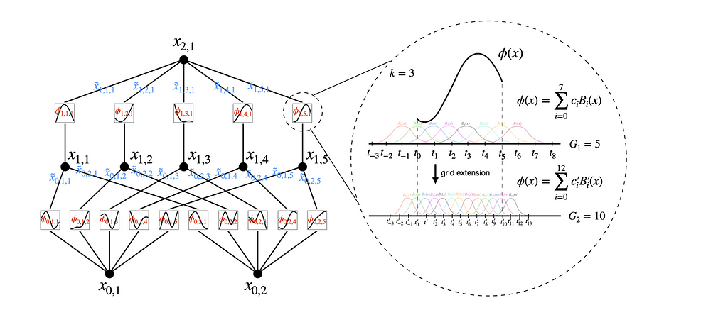
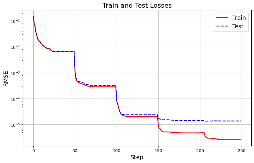
Now let’s build a KAN model and train it on the dataset. We will start with a coarse grid (5 points) and gradually refine it (up to 100 points). This improves the model’s accuracy by capturing finer details in the data.
for i in range(grids.shape[0]): if i == 0: model = KAN(width=[2, 1, 1], grid=grids[i], k=k) else: model = KAN(width=[2, 1, 1], grid=grids[i], k=k).initialize_from_another_model(model, dataset['train_input']) results = model.train(dataset, opt="LBFGS", steps=steps, stop_grid_update_step=30) train_losses_kan += results['train_loss'] test_losses_kan += results['test_loss']
print(f"Train RMSE: {results['train_loss'][-1]:.8f} | Test RMSE: {results['test_loss'][-1]:.8f}")
In this example, we define an array called grids with values [5, 10, 20, 50, 100]. We iterate over these grids to fit models sequentially, meaning each new model is initialized using the previous one.
For each iteration, we define a model with k=3, where k is the order of the B-spline. We set the number of training steps (or epochs) to 50. The model’s architecture consists of an input layer with 2 nodes, one hidden layer with 1 node, and an output layer with 1 node. We use the LFGBS optimizer for training.
Here are the training and test losses during the training process:
KAN Train and Test Losses Plot — Image by Author
Let’s now define and train a traditional MLP for comparison.
epochs = 250 for epoch in range(epochs): optimizer.zero_grad() output = model(dataset['train_input']).squeeze() loss = criterion(output, dataset['train_label']) loss.backward() optimizer.step() train_loss_mlp.append(loss.item()**0.5)
# Test the model model.eval() with torch.no_grad(): output = model(dataset['test_input']).squeeze() loss = criterion(output, dataset['test_label']) test_loss_mlp.append(loss.item()**0.5)
print(f'Epoch {epoch+1}/{epochs}, Train Loss: {train_loss_mlp[-1]:.2f}, Test Loss: {test_loss_mlp[-1]:.2f}', end='r')
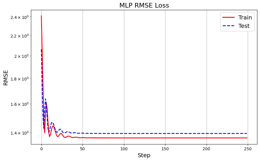
We use mean squared error (MSE) loss and Adam optimizer, and train the model for 250 epochs, recording the training and testing losses.
This is what the train and test RMSE look like in MLP:
MLP Train and Test Losses Plot — Image by Author
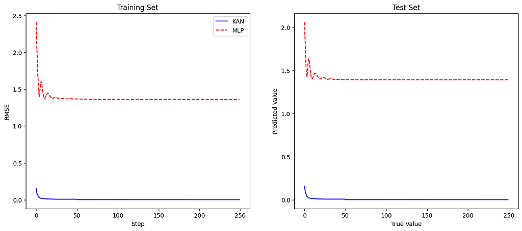
Let’s put side to side the loss plots for a comparison:
KAN vs MLP training losses plot (left) and test losses plot (right) — Image by Author
The plot shows that the KAN model achieves lower training RMSE than the MLP model, indicating better function-fitting capability. Similarly, the KAN model outperforms the MLP on the test set, demonstrating its superior generalization ability.
This example illustrates how KANs can more accurately fit complex functions than traditional MLPs, thanks to their flexible and adaptive structure. By refining the grid and employing learnable univariate functions on the edges, KANs capture intricate patterns in the data that MLPs may miss, leading to improved performance in function-fitting tasks.
Does this mean we should switch to KAN models permanently? Not necessarily.
KANs showed great results in this example, but when I tested them on other scenarios with real data, MLPs often performed better. One thing you’ll notice when working with KAN models is their sensitivity to hyperparameter optimization. Also, KANs have primarily been tested using spline functions, which work well for smoothly varying data like our example but might not perform as well in other situations.
In summary, KANs are definitely intriguing and have a lot of potential, but they need more study, especially regarding different datasets and the algorithm’s inner workings, to really make them work effectively.
5: Advantages of KANs
Accuracy
One of the standout advantages of Kolmogorov-Arnold Networks (KANs) is their ability to achieve higher accuracy with fewer parameters compared to traditional Multi-Layer Perceptrons (MLPs). This is primarily due to the learnable activation functions on the edges, which allow KANs to better capture complex patterns and relationships in the data.
Unlike MLPs that use fixed activation functions at each node, KANs use univariate functions on the edges, making the network more flexible and capable of fine-tuning its learning process to the data.
Because KANs can adjust the functions between layers dynamically, they can achieve comparable or even superior accuracy with a smaller number of parameters. This efficiency is particularly beneficial for tasks with limited data or computational resources.
Interpretability
KANs offer significant improvements in interpretability over traditional MLPs. This enhanced interpretability is crucial for applications where understanding the decision-making process is as important as the outcome.
KANs can be simplified through techniques like sparsification and pruning, which remove unnecessary functions and parameters. These techniques not only improve interpretability but also enhance the network’s performance by focusing on the most relevant components.
For some functions, it is possible to identify symbolic forms of the activation functions, making it easier to understand the mathematical transformations within the network.
Scalability
KANs exhibit faster neural scaling laws compared to MLPs, meaning they improve more rapidly as the number of parameters increases.
KANs benefit from more favorable scaling laws due to their ability to decompose complex functions into simpler, univariate functions. This allows them to achieve lower error rates with increasing model complexity more efficiently than MLPs.
KANs can start with a coarser grid and extend it to finer grids during training, which helps in balancing computational efficiency and accuracy. This approach allows KANs to scale up more gracefully than MLPs, which often require complete retraining when increasing model size.
Conclusion
Kolmogorov-Arnold Networks (KANs) present a groundbreaking alternative to traditional Multi-Layer Perceptrons (MLPs), offering several key innovations that address the limitations of their predecessors. By leveraging learnable activation functions on the edges rather than fixed functions at the nodes, KANs introduce a new level of flexibility and adaptability. This structural change leads to:
Enhanced Accuracy: KANs achieve higher accuracy with fewer parameters, making them more efficient and effective for a wide range of tasks.
Improved Interpretability: The ability to visualize and simplify KANs aids in understanding the decision-making process, which is crucial for critical applications in healthcare, finance, and autonomous systems.
Better Scalability: KANs exhibit faster neural scaling laws, allowing them to handle increasing complexity more gracefully than MLPs.
The introduction of Kolmogorov-Arnold Networks marks an exciting development in the field of neural networks, opening up new possibilities for AI and machine learning.
The world of large language models (LLMs) is constantly evolving, with new advancements emerging rapidly. One exciting area is the development of multi-modal LLMs (MLLMs), capable of understanding and interacting with both texts and images. This opens up a world of possibilities for tasks like document understanding, visual question answering, and more.
I recently wrote a general post about one such model that you can check out here:
But in this one, we’ll explore a powerful combination: the InternVL model and the QLoRA fine-tuning technique. We will focus on how we can easily customize such models for any specific use-case. We’ll use these tools to create a receipt understanding pipeline that extracts key information like company name, address, and total amount of purchase with high accuracy.
Understanding the Task and Dataset
This project aims to develop a system that can accurately extract specific information from scanned receipts, using InternVL’s capabilities. The task presents a unique challenge, requiring not only robust natural language processing (NLP) but also the ability to interpret the visual layout of the input image. This will enable us to create a single, OCR-free, end-to-end pipeline that demonstrates strong generalization across complex documents.
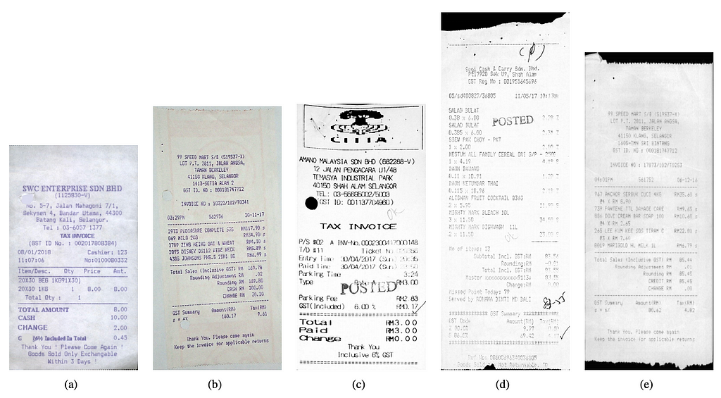
To train and evaluate our model, we’ll use the SROIE dataset. SROIE provides 1000 scanned receipt images, each annotated with key entities like:
We will evaluate the performance of our model using a fuzzy similarity score, a metric that measures the similarity between predicted and ground truth entities. This metric ranges from 0 (irrelevant results) to a 100 (perfect predictions).
InternVL: A Multi-modal Powerhouse
InternVL is a family of multi-modal LLMs from the OpenGVLab, designed to excel in tasks involving image and text. Its architecture combines a vision model (like InternViT) with a language model (like InternLM2 or Phi-3). We’ll focus on the Mini-InternVL-Chat-2B-V1–5 variant, a smaller version that is well-suited for running on consumer-grade GPUs.
InternVL’s key strengths:
Efficiency: Its compact size allows for efficient training and inference.
Accuracy: Despite being smaller, it achieves competitive performance in various benchmarks.
Multi-modal Capabilities: It seamlessly combines image and text understanding.
Demo: You can explore a live demo of InternVL here.
Finetuning with QLoRA: A Memory-Efficient Approach
To further boost our model’s performance, we’ll use QLoRA which is a fine-tuning technique that significantly reduces memory consumption while preserving performance. Here’s how it works:
Quantization: The pre-trained LLM is quantized to 4-bit precision, reducing its memory footprint.
Low-Rank Adapters (LoRA): Instead of modifying all parameters of the pre-trained model, LoRA adds small, trainable adapters to the network. These adapters capture task-specific information without requiring changes to the main model.
Efficient Training: The combination of quantization and LoRA enables efficient fine-tuning even on GPUs with limited memory.
Code Walk-through: Baseline Performance
Let’s dive into the code. First, we’ll assess the baseline performance of Mini-InternVL-Chat-2B-V1–5 without any fine-tuning:
# single-round single-image conversation question = ( "Extract the company, date, address and total in json format." "Respond with a valid JSON only." ) # print(model) response = model.chat(tokenizer, pixel_values, question, generation_config)
print(response)
The result:
```json
{
  "company": "SAM SAM TRADING CO",
  "date": "Fri, 29-12-2017",
  "address": "67, JLN MENHAW 25/63 TNN SRI HUDA, 40400 SHAH ALAM",
  "total": "RM 14.10"
}
```
This code:
Loads the model from the Hugging Face hub.
Loads a sample receipt image and converts it to a tensor.
Formulates a question asking the model to extract relevant information from the image.
Runs the model and outputs the extracted information in JSON format.
This zero-shot evaluation shows impressive results, achieving an average fuzzy similarity score of 74.24%. This demonstrates InternVL’s ability to understand receipts and extract information with no fine-tuning.
Fine-tuning: Enhancing Performance with QLoRA
To further boost accuracy, we’ll fine-tune the model using QLoRA. Here’s how we implement it:
# set the max number of tiles in `max_num` img_context_token_id = tokenizer.convert_tokens_to_ids(IMG_CONTEXT_TOKEN) print("img_context_token_id", img_context_token_id) model.img_context_token_id = img_context_token_id
{ "company": "YONG TAT HARDWARE TRADING", "date": "13/03/2018", "address": "NO 4, JALAN PERUBANAN 10, TAMAN AIR BIRU, 81700 PASIR GUDANG, JOHOR", "total": "72.00" }
Results and Conclusion
After fine-tuning with QLoRA, our model achieves a remarkable 95.4% fuzzy similarity score, a significant improvement over the baseline performance (74.24%). This demonstrates the power of QLoRA in boosting model accuracy without requiring massive computing resources (15 min training on 600 samples on a RTX 3080 GPU).
We’ve successfully built a robust receipt understanding pipeline using InternVL and QLoRA. This approach showcases the potential of multi-modal LLMs for real-world tasks like document analysis and information extraction. In this example use-case, we gained 30 points in prediction quality using a few hundred examples and a few minutes of compute time on a consumer GPU.
You can find the full code implementation for this project here.
The development of multi-modal LLMs is only just beginning, and the future holds exciting possibilities. The area of automated document processing has immense potential in the era of MLLMs. These models can revolutionize how we extract information from contracts, invoices, and other documents, requiring minimal training data. By integrating text and vision, they can analyze the layout of complex documents with unprecedented accuracy, paving the way for more efficient and intelligent information management.
The future of AI is multi-modal, and InternVL and QLoRA are powerful tools to help us unlock its potential on a small compute budget.
In early 2013, authors from Université Côte d’Azur and Max-Planck-Institut für Informatik published a paper titled “3D Gaussian Splatting for Real-Time Field Rendering.”¹ The paper presented a significant advancement in real-time neural rendering, surpassing the utility of previous methods like NeRF’s.² Gaussian splatting not only reduced latency but also matched or exceeded the rendering quality of NeRF’s, taking the world of neural rendering by storm.
Gaussian splatting, while effective, can be challenging to understand for those unfamiliar with camera matrices and graphics rendering. Moreover, I found that resources for implementing gaussian splatting in Python are scarce, as even the author’s source code is written in CUDA! This tutorial aims to bridge that gap, providing a Python-based introduction to gaussian splatting for engineers versed in python and machine learning but less experienced with graphics rendering. The accompanying code on GitHub demonstrates how to initialize and render points from a COLMAP scan into a final image that resembles the forward pass in splatting applications(and some bonus CUDA code for those interested). This tutorial also has a companion jupyter notebook (part_1.ipynb in the GitHub) that has all the code needed to follow along. While we will not build a full gaussian splat scene, if followed, this tutorial should equip readers with the foundational knowledge to delve deeper into splatting technique.
To begin, we use COLMAP, a software that extracts points consistently seen across multiple images using Structure from Motion (SfM).³ SfM essentially identifies points (e.g., the top right edge of a doorway) found in more than 1 picture. By matching these points across different images, we can estimate the depth of each point in 3D space. This closely emulates how human stereo vision works, where depth is perceived by comparing slightly different views from each eye. Thus, SfM generates a set of 3D points, each with x, y, and z coordinates, from the common points found in multiple images giving us the “structure” of the scene.
In this tutorial we will use a prebuilt COLMAP scan that is available for download here (Apache 2.0 license). Specifically we will be using the Treehill folder within the downloaded dataset.
The image along with all the points extracted from all images fed to COLMAP. See sample code below or in part_1.ipynb to understand the process. Apache 2.0 license.
The folder consists of three files corresponding to the camera parameters, the image parameters and the actual 3D points. We will start with the 3D points.
The points file consists of thousands of points in 3D along with associated colors. The points are centered around what is called the world origin, essentially their x, y, or z coordinates are based upon where they were observed in reference to this world origin. The exact location of the world origin isn’t crucial for our purposes, so we won’t focus on it as it can be any arbitrary point in space. Instead, its only essential to know where you are in the world in relation to this origin. That is where the image file becomes useful!
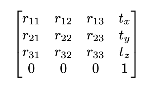
Broadly speaking the image file tells us where the image was taken and the orientation of the camera, both in relation to the world origin. Therefore, the key parameters we care about are the quaternion vector and the translation vector. The quaternion vector describes the rotation of the camera in space using 4 distinct float values that can be used to form a rotation matrix (3Blue1Brown has a great video explaining exactly what quaternions are here). The translation vector then tells us the camera’s position relative to the origin. Together, these parameters form the extrinsic matrix, with the quaternion values used to compute a 3×3 rotation matrix (formula) and the translation vector appended to this matrix.
A typical “extrinsic” matrix. By combining a 3×3 rotation matrix and a 3×1 translation vector we are able to translate coordinates from the world coordinate system to our camera coordinate system. Image by author.
The extrinsic matrix translates points from world space (the coordinates in the points file) to camera space, making the camera the new center of the world. For example, if the camera is moved 2 units up in the y direction without any rotation, we would simply subtract 2 units from the y-coordinates of all points in order to obtain the points in the new coordinate system.
When we convert coordinates from world space to camera space, we still have a 3D vector, where the z coordinate represents the depth in the camera’s view. This depth information is crucial for determining the order of splats, which we need for rendering later on.
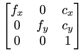
We end our COLMAP examination by explaining the camera parameters file. The camera file provides parameters such as height, width, focal length (x and y), and offsets (x and y). Using these parameters, we can compose the intrinsic matrix, which represents the focal lengths in the x and y directions and the principal point coordinates.
If you are completely unfamiliar with camera matrices I would point you to the First Principles of Computer Vision lectures given by Shree Nayar. Specially the Pinhole and Prospective Projection lecture followed by the Intrinsic and Extrinsic matrix lecture.
The typical intrinsic matrix. Representing the focal length in the x and y direction, along with the principal point coordinates. Image by author.
The intrinsic matrix is used to transform points from camera coordinates (obtained using the extrinsic matrix) to a 2D image plane, ie. what you see as your “image.” Points in camera coordinates alone do not indicate their appearance in an image as depth must be reflected in order to assess exactly what a camera will see.
To convert COLMAP points to a 2D image, we first project them to camera coordinates using the extrinsic matrix, and then project them to 2D using the intrinsic matrix. However, an important detail is that we use homogeneous coordinates for this process. The extrinsic matrix is 4×4, while our input points are 3×1, so we stack a 1 to the input points to make them 4×1.
Here’s the process step-by-step:
Transform the points to camera coordinates: multiply the 4×4 extrinsic matrix by the 4×1 point vector.
Transform to image coordinates: multiply the 3×4 intrinsic matrix by the resulting 4×1 vector.
This results in a 3×1 matrix. To get the final 2D coordinates, we divide by the third coordinate of this 3×1 matrix and obtain an x and y coordinate in the image! You can see exactly how this should look about for image number 100 and the code to replicate the results is shown below.
def get_intrinsic_matrix( f_x: float, f_y: float, c_x: float, c_y: float ) -> torch.Tensor: """ Get the homogenous intrinsic matrix for the camera """ return torch.Tensor( [ [f_x, 0, c_x, 0], [0, f_y, c_y, 0], [0, 0, 1, 0], ] )
def get_extrinsic_matrix(R: torch.Tensor, t: torch.Tensor) -> torch.Tensor: """ Get the homogenous extrinsic matrix for the camera """ Rt = torch.zeros((4, 4)) Rt[:3, :3] = R Rt[:3, 3] = t Rt[3, 3] = 1.0 return Rt
def project_points( points: torch.Tensor, intrinsic_matrix: torch.Tensor, extrinsic_matrix: torch.Tensor ) -> torch.Tensor: """ Project the points to the image plane
To review, we can now take any set of 3D points and project where they would appear on a 2D image plane as long as we have the various location and camera parameters we need! With that in hand we can move forward with understanding the “gaussian” part of gaussian splatting in part 2.
Kerbl, Bernhard, et al. “3d gaussian splatting for real-time radiance field rendering.” ACM Transactions on Graphics 42.4 (2023): 1–14.
Mildenhall, Ben, et al. “Nerf: Representing scenes as neural radiance fields for view synthesis.” Communications of the ACM 65.1 (2021): 99–106.
Snavely, Noah, Steven M. Seitz, and Richard Szeliski. “Photo tourism: exploring photo collections in 3D.” ACM siggraph 2006 papers. 2006. 835–846.
Barron, Jonathan T., et al. “Mip-nerf 360: Unbounded anti-aliased neural radiance fields.” Proceedings of the IEEE/CVF Conference on Computer Vision and Pattern Recognition. 2022.
We use cookies on our website to give you the most relevant experience by remembering your preferences and repeat visits. By clicking “Accept”, you consent to the use of ALL the cookies.
This website uses cookies to improve your experience while you navigate through the website. Out of these, the cookies that are categorized as necessary are stored on your browser as they are essential for the working of basic functionalities of the website. We also use third-party cookies that help us analyze and understand how you use this website. These cookies will be stored in your browser only with your consent. You also have the option to opt-out of these cookies. But opting out of some of these cookies may affect your browsing experience.
Necessary cookies are absolutely essential for the website to function properly. These cookies ensure basic functionalities and security features of the website, anonymously.
Cookie
Duration
Description
cookielawinfo-checkbox-analytics
11 months
This cookie is set by GDPR Cookie Consent plugin. The cookie is used to store the user consent for the cookies in the category "Analytics".
cookielawinfo-checkbox-functional
11 months
The cookie is set by GDPR cookie consent to record the user consent for the cookies in the category "Functional".
cookielawinfo-checkbox-necessary
11 months
This cookie is set by GDPR Cookie Consent plugin. The cookies is used to store the user consent for the cookies in the category "Necessary".
cookielawinfo-checkbox-others
11 months
This cookie is set by GDPR Cookie Consent plugin. The cookie is used to store the user consent for the cookies in the category "Other.
cookielawinfo-checkbox-performance
11 months
This cookie is set by GDPR Cookie Consent plugin. The cookie is used to store the user consent for the cookies in the category "Performance".
viewed_cookie_policy
11 months
The cookie is set by the GDPR Cookie Consent plugin and is used to store whether or not user has consented to the use of cookies. It does not store any personal data.
Functional cookies help to perform certain functionalities like sharing the content of the website on social media platforms, collect feedbacks, and other third-party features.
Performance cookies are used to understand and analyze the key performance indexes of the website which helps in delivering a better user experience for the visitors.
Analytical cookies are used to understand how visitors interact with the website. These cookies help provide information on metrics the number of visitors, bounce rate, traffic source, etc.
Advertisement cookies are used to provide visitors with relevant ads and marketing campaigns. These cookies track visitors across websites and collect information to provide customized ads.