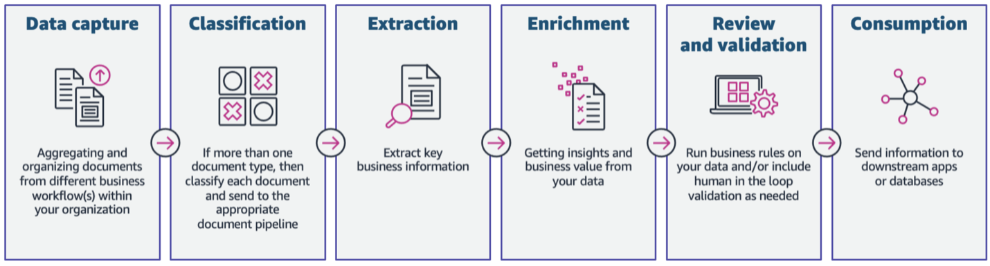
This post explains a generative artificial intelligence (AI) technique to extract insights from business emails and attachments. It examines how AI can optimize financial workflow processes by automatically summarizing documents, extracting data, and categorizing information from email attachments. This enables companies to serve more clients, direct employees to higher-value tasks, speed up processes, lower expenses, enhance data accuracy, and increase efficiency.
How to Find and Solve Valuable Generative-AI Use Cases
80% of AI projects fail due to poor use cases or technical knowledge. Gen AI reduced complexity, and now we must pick the right battles.
“Paperclips & Friends” company wants to jump on the AI hype train. How far will they ride?
It has become apparent that AI projects are hard. Some estimate that 80% of the AI projects fail. Still, generative AI is here to stay, and companies are searching for how to apply it to their operations. AI projects fail, because they fail to deliver value. The root cause of failure is applying AI to the wrong use cases. The solution for finding the right use cases is with three measures:
Measure the problem magnitude
Measure the solution accuracy retrospectively
Measure the solution accuracy in real time
These steps should be investigated sequentially. If the problem magnitude is not big enough to bring the needed value, do not build. If the solution accuracy on historical data is not high enough, do not deploy. If the real-time accuracy is not high enough, adjust the solution.
Each Measure stage must be passed to move to the next stage.
I will be discussing generative AI instead of AI in general. Generative AI is a small subfield of AI. With general AI projects the goal is to find a model to approximate how the data is generated — you must have high proficiency in understanding different machine learning algorithms and data processing. With generative AI the model is given, LLM (e.g. chatGPT), and the goal is to use the existing model to solve some business problem. The latter requires less technical skills, and more problem solving knowledge. Generative AI use cases are much easier to implement and validate, as the step of creating the algorithm is left out, and the data (text) is (relatively) standardized.
Measure the problem magnitude
Every person can identify problems in their daily work. The challenge lies in determining which issues are significant enough to be solved and where AI could and should be applied.
Instead of going through all subjective problems and finding data to validate their existence, we can focus on processes that generate textual data. This approach narrows the scope to measurable problems,where AI and automation can add demonstrable value.
Concretely, instead of asking the customer support specialist “What problems are there in your work?”, we should measure where the employee spends the most time. Let’s go through this with an example.
Paperclips & Friends is a paper clip company. Look at those happy faces.
Paperclips & Friends (P&F) is a company that makes paper clips. They have a support channel #P&FSupport, where customers discuss issues around paper clips. P&F responds to customer questions on time, but the channel keeps getting busier. The customer support specialists hear about ChatGPT and want it to help with customer questions.
The paper clip customer support experts are tired of all the customer questions.
Before the data science team of P&F starts solving the issue, they measure the number of incoming questions to understand the magnitude of the problem. They notice hundreds and hundreds of inquiries, daily.
The data science team develops a RAG chatbot using ChatGPT and P&F internal documentation. They release the chatbot to be tested by the customer support specialists and receive mixed feedback. Some experts love the solution and mention that it solves most of the issues, while others criticize it, claiming it provides no value.
The P&F data science team faces a challenge — who speaks the truth? Is the chatbot any good? Then, they remember the second Measure:
“Measure the solution accuracy retrospectively”
NOTE: it is crucial to verify can the root cause be solved. If Paperclips & Friends found out, that 90% of the support channel messages were related to unclear usage instructions, P&F could create a chatbot for answering those messages. However, the customer wouldn’t have sent the question in the first place, if P&F included a simple instruction guide with the paperclip shipment.
Illustration of the P&F data science team doing their best to build a chatbot.
Measure the solution accuracy retrospectively
The P&F data science team faces a challenge: They must weigh each expert opinion equally, but can’t satisfy everyone. Instead of focusing on expert subjective opinions, they decide to evaluate the chatbot on historical customer questions. Now experts do not need to come up with questions to test the chatbot, bringing the evaluation closer to real-world conditions. The initial reason for involving experts, after all, was their better understanding of real customer questions compared to the P&F data science team.
It turns out that commonly asked questions for P&F are related to paper clip technical instructions. P&F customers want to know detailed technical specifications of the paper clips. P&F has thousands of different paper clip types, and it takes a long time for customer support to answer the questions.
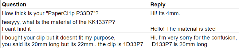
Understanding the test-driven development, the data science team creates a dataset from the conversation history, including the customer question and customer support reply:
Dataset gathered from Paperclips & Friends discord channel.
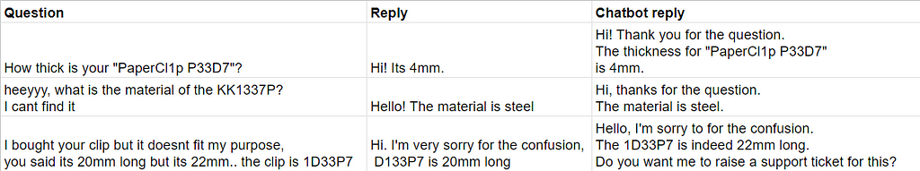
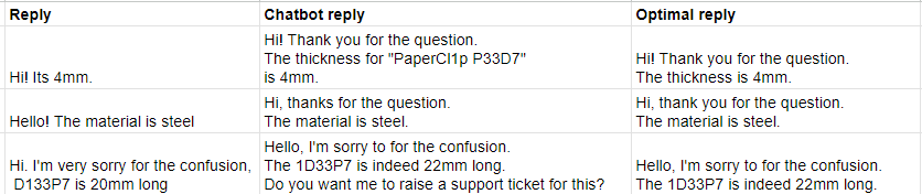
Having a dataset of questions and answers, P&F can test and evaluate the chatbot’s performance retrospectively. They create a new column, “Chatbot reply”, and store the chatbot example replies to the questions.
Augmented dataset with proposed chatbot answer.
We can have the experts and GPT-4 evaluate the quality of the chatbot’s replies. The ultimate goal is to automate the chatbot accuracy evaluation by utilizing GPT-4. This is possible ifexperts and GPT-4 evaluate the replies similarly.
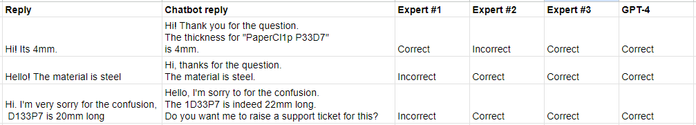
Experts create a new Excel sheet with each expert’s evaluation, and the data science team adds the GPT-4 evaluation.
Augmented dataset with expert and GPT-4 evaluations.
There are conflicts on how different experts evaluate the same chatbot replies. GPT-4 evaluates similarly to expert majority voting, which indicates that we could do automatic evaluations with GPT-4. However, each expert’s opinion is valuable, and it’s important to address the conflicting evaluation preferences among the experts.
P&F organizes a workshop with the experts to create golden standard responses to the historical question dataset
The golden standard dataset for evaluation.
and evaluationbest practice guidelines, to which all experts agree.
Evaluation “best practices guidelines” for the chatbot as defined by customer support specialists.
With the insights from the workshop, the data science team can create a more detailed evaluation prompt for the GPT-4 that covers edge cases (i.e. “chatbot should not ask to raise support tickets”). Now the experts can use time to improve the paper clip documentation and define best practices, instead of laborious chatbot evaluations.
By measuring the percentage of correct chatbot replies, P&F can decide whether they want to deploy the chatbot to the support channel. They approve the accuracy and deploy the chatbot.
Measure the solution accuracy in real-time
Finally, it’s time to save all the chatbot responses and calculate how well the chatbot performs to solve real customer inquiries. As the customer can directly respond to the chatbot, it is also important to record the response from the customer, to understand the customer’s sentiment.
The same evaluation workflow can be used to measure the chatbot’s success factually, without the ground truth replies. But now the customers are getting the initial reply from a chatbot, and we do not know if the customers like it. We should investigate how customers react to the chatbot’s replies. We can detect negative sentiment from the customer’s replies automatically, and assign customer support specialists to handle angry customers.
Conclusion
In this short article, I explained three steps to avoid failing your AI project:
Measure the problem magnitude
Measure the solution accuracy retrospectively
Measure the solution accuracy in real-time
The first two steps are by far the most crucial and are the primary reasons why many projects fail. While it is possible to succeed without measuring the problem’s magnitude or the solution’s accuracy, subjective estimates are generally flawed due to hundreds of human biases. Correctly designed data-driven approaches almost always give better results.
On Pixel Transformer and Ultra-long Sequence Distributed Transformer
Have you ever wondered why the Vision Transformer (ViT) uses 16*16 size patches as input tokens?
It all dates back to the earlier days of the Transformers. The original Transformer model was proposed in 2017 and only works with natural language data. When the BERT model was released in 2018, it could only handle a max token sequence of length 512. Later in 2020, when GPT-3 was released, it could handle a sequence of lengths 2048 and 4096 at 3.5. All these models showed amazing performance in handling sequence-to-sequence and text-generation tasks.
However, these sequences were too short for images when tokens were taken at the pixel level. For example, in Cifar-100, the image size is 32* 32 = 1024 pixels. In ImageNet, the image size is 224* 224 = 50176 pixels. The sequence length would be an immediate barrier if the transformer were directly applied to the pixel level.
The ViT paper was released in 2020. It proposed using patches rather than pixels as the input tokens. For an image of size 224* 224, using a patch size of 16* 16, the sequence length would be largely reduced to 196, which perfectly solved the issue.
However, the issue was only partially solved. For tasks requiring features of finer details, different approaches have to be utilized to get the pixel-level accuracy back. Segformer proposed to fuse features from hierarchical transformer encoders of different resolutions. SwinIR had to combine CNN with multiple levels of skip connection around the transformer module for fine-grained feature extraction. The Swin Transformer, a model for universal computer vision tasks, started with a patch size 4*4 in each local window and then gradually built toward the global 16*16 patch size to obtain both globality and granularity. Intrinsically, these efforts pointed to one fact — simply using the 16*16 size patch is insufficient.
The natural question is, can “pixel” be used as a direct token for transformers? The question further splits into two: 1. Is it possible to feed an ultralong sequence (e.g., 50k) to a transformer? 2. does feeding pixels as tokens provide more information than patches?
In this article, I will summarize two recent papers: 1. Pixel Transformer, a technical report released by Meta AI last week, comparing pixel-wise tokens and patch-wise tokens to transformer models from the perspective of reducing the inductive bias of locality on three different tasks: image classification, pre-training, and generation. 2. Ultra-long sequence distributed transformer: by distributing the query vector, the authors showed the possibility to scale an input sequence of length 50k on 3k GPUs.
Pixel Transformer (PiT) — from an inductive bias perspective
Meta AI released The technical report last week on arXiv: “An image is worth more than 16*16 patches”. Instead of proposing a novel method, the technical report answered a long-lasting question: Does it make sense to use pixels instead of patches as input tokens? If so, why?
The paper took the perspective of the Inductive Bias of Locality. According to K. Murphy’s well-known machine learning book, inductive bias is the “assumptions about the nature of the data distribution.” In the early “non-deep learning” era, the inductive bias was more “feature-related,” coming from the manual feature engineered for specific tasks. This inductive bias was not a bad thing, especially for specific tasks in which very good prior knowledge from human experts is gained, making the engineered features very useful. However, from the generalization perspective, the engineered features are very hard to generalize to universal tasks, like general image classification and segmentation.
But beyond feature bias, the architecture itself contains inductive bias as well. The ViT is a great example showing less inductive bias than CNN models in terms of architecture hierarchy, propagation uniformness, representation scale, and attention locality. See my previous medium post for a detailed discussion. But still, ViT remains a special type of inductive bias — locality. When the ViT processes a sequence of patch tokens, the pixels within the same patch are naturally treated by the model differently than those from different patches. And that’s where the locality comes from.
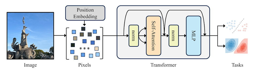
So, is it possible to remove the inductive bias of locality further? The answer is yes. The PiT proposed using the “pixel set” as input with different position embedding (PE) strategies: sin-cos, learnt, and none. It showed superior performance over ViT on supervised, self-supervised, and generation tasks. The proposed pipeline is shown in the figure below.
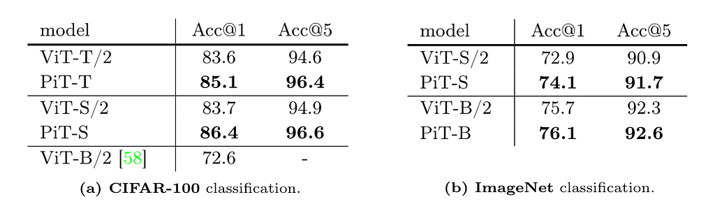
The idea seems simple and straightforward, and the authors claim they are “not introducing a new method” here. But still, the PiT shows great potential. On CIFAR-100 and ImageNet (reduced input size to 28*28) supervised classification tasks, the classification accuracy increased by more than 2% over ViT. See the table below.
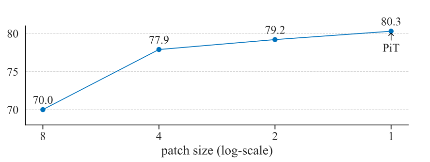
Similar improvement was also observed in self-supervised learning tasks and image generation tasks. What’s more, the authors also showed the trend of a performance increase when reducing the patch size from 8*8 to 1*1 (single pixel) as below:
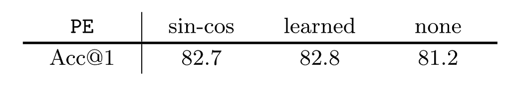
As pointed out in this research paper, positional encoding is a prerequisite in transformer-based models for input token sequence ordering and improving accuracy. However, the PiT shows that even after dropping the PE, the model performance drops is minimal:
PiT performance using three different PE: 1. fixed sin-cos PE; 2. learnable PE; 3. no PE. Image source: https://arxiv.org/pdf/2406.09415
Why drop the positional encoding? It is not only because dropping the positional encoding means a good reduction of the locality bias. If we think of self-attention computation in a distributed manner, it will largely reduce the cross-device communication effort, which we’ll discuss in detail in the next section.
Ultra-long Sequences Transformers — a distributed query vector solution
The inductive bias of locality only told part of the story. If we look closely at the results in the PiT paper, we see that the experiments were limited to 28*28 resized images due to the computational limit. But the real world rarely uses images of such a small size. So the natural question is, even though PiT might be useful and outperform ViT, could it work on natural images of standard resolution, e.g., 244*244?
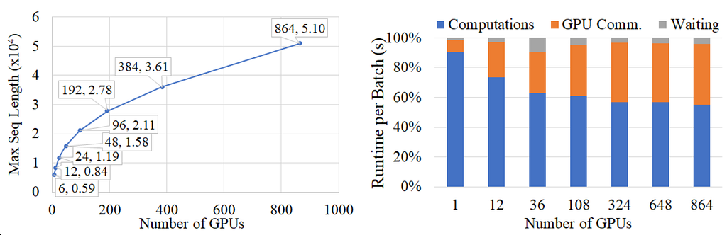
The paper “Ultra-long sequence distributed transformer,” released in 2023, answers the question. The paper proposed a solution to scale the transformer computation of a 50k-long sequence onto 3k GPUS.
Original transformer, baseline parallelization, and proposed ultra-long sequence transformer. Image source: https://arxiv.org/pdf/2311.02382
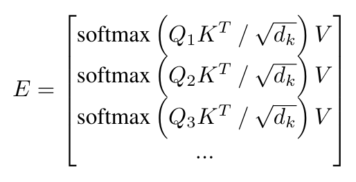
The idea is simple: The transformer’s bottleneck is self-attention computation. To ensure global attention computation, the proposed method only distributes the query vectors across different devices while maintaining the same copies of key and value vectors on all devices.
The equation for distributing self-attention calculation. The core idea is to distribute Q and keep the same copies of K and V. Image source: https://arxiv.org/pdf/2311.02382
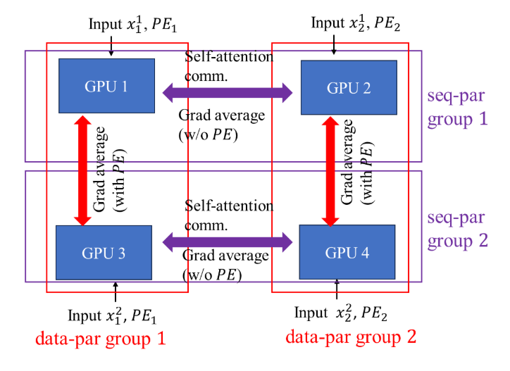
Positional Encoding-aware double gradient averaging. For architectures with learnable positional encoding parameters, gradient backpropagation is related to the positional encoding distribution. So, the authors proposed the double gradient averaging technique: when a gradient average is performed on two different segments from the same sequence, no positional encoding is involved, but when the corresponding segments from two sequences need to average gradients, the positional encoding parameters will be synced.
When we combine these two papers, things become interesting. Reducing the inductive bias not only helps with model performance but also plays a crucial role in distributed computation.
Inductive bias of locality and device communication. The PiT paper shows the potential of building a positional encoding-free model by removing the locality bias. Furthermore, if we look at things from the distributed computing perspective, reducing the need for PE could further reduce the communication burden across devices.
Inductive bias of locality in distributed sequence computation. Distributing self-attention on multi-GPUs means the query vector is segment-based. There is a natural locality bias if the segment depends on contiguous tokens. The PiT computes on a “token set, ” meaning there is no need for continuous segments, and it will make the query vector bias-free.
References:
Nguyen et al., An Image is Worth More Than 16×16 Patches: Exploring Transformers on Individual Pixels. arXiv preprint 2024.
Wang et al., Ultra long sequence distributed transformer. arXiv preprint 2023.
Keles et al., On the computational complexity of self-attention. ALT 2023.
Jiang et al. The encoding method of position embeddings in vision transformer. Journal of Visual Communication and Image Representation. 2022.
Xie et al., SegFormer: Simple and efficient design for semantic segmentation with transformers. NeurIPS 2021. Github: https://github.com/NVlabs/SegFormer
Keras is Back!! First released in 2015 as a high-level Python library for training ML models, Keras grew in popularity due to its clean and simple APIs. Contrary to the ML frameworks of the time, with their awkward and clunky APIs, Keras lowered the entry bar for many incumbent ML developers (the author included). But somewhere along the way the use of Keras became virtually synonymous with TensorFlow development. Consequently, when developers began to turn to alternative frameworks, the relative popularity of Keras began to decline. But now, following a “complete rewrite”, Keras has returned. And with its shiny new engine and its renewed commitment to multi-backend support, it vies to return to its former glory.
In this post we will take a new look at Keras and assess its value offering in the current era of AI/ML development. We will demonstrate through example its ease of use and make note of its shortcomings. Importantly, this post is not intended to be an endorsement for or against the adoption of Keras (or any other framework, library, service, etc.). As usual, the best decision for your project development will depend on a great many details, many of which are beyond the scope of this post.
The recent release of Google’s family of open sourced NLP models known as Gemma, and the inclusion of Keras 3 as a core component of the API, offers us an opportunity to evaluate Keras’s goodness and could serve as a great opportunity for its resurgence.
Why Use Keras 3?
In our view, the most valuable feature offered by Keras 3 is its multi-framework support. This may surprise some readers who may recall Keras’s distinctiveness to be its user experience. Keras 3 advertises itself, as “simple”, “flexible”, and being “designed for human beings, not machines”. And indeed, it owes its early successes and meteoric rise in popularity to its user experience. But it is now 2024 and there are many high-level deep learning APIs offering “reduced cognitive load”. In our view, the user experience, as good as it may be, is no longer a sufficient motivator to consider Keras over its alternatives. Its multi-framework support is.
The Merits of Multi-Framework Support
Keras 3 supports multiple backends for training and running its models. At the time of this writing, these include JAX, TensorFlow, and PyTorch. The Keras 3 announcement does a pretty good job of explaining the advantages of this feature. We will expand on the documented benefits and add some of our own flavor.
Avoid the difficulty of choosing an AI/ML framework: Choosing an AI/ML framework is probably one of the most important decisions you will need to make as an ML developer. It is also one of the hardest. There are many considerations that need to factor into this decision. These include user experience, API coverage, programmability, debuggability, the formats and types of input data that are supported, conformance with other components on the development pipeline (e.g., restrictions that may be imposed by the model deployment phase), and, perhaps most importantly, runtime performance. As we have discussed in many of our previous posts (e.g., here), AI/ML model development can be extremely expensive and the overall impact on cost of even the smallest speed-up due to the choice of framework can be dramatic. In fact, in many cases it may warrant the overhead of porting your model and code to a different framework and/or even maintaining support for multiple frameworks.
The problem is that it is extremely difficult, if not impossible, to know which framework will be most optimal for your model before you start your development. Moreover, even once you have committed to one framework, you will want to stay on top of the evolution and development of all frameworks and to continuously assess potential opportunities to improve your model and/or reduce the cost of development. The landscape of AI/ML development is extremely dynamic with optimizations and enhancements being designed and developed on a consistent basis. You will not want to fall behind.
Keras 3 solves the framework selection problem by enabling you to develop your model without committing to an underlying backend. The option to toggle between multiple framework-backends allows you to focus on the model definition and, once complete, choose the backend that best suits your needs. And even as the properties of the ML project change or the supported frameworks evolve, Keras 3 enables you to easily assess the impact of changing the backend.
Putting it colloquially, you could say that Keras 3 helps humans avoid one of the things they hate doing most — making decisions and committing to them. But humor aside, AI/ML model development using Keras 3 can certainly prevent you from choosing and being stuck with a suboptimal framework.
Enjoy the best of all worlds: PyTorch, TensorFlow, and JAX, each have their own unique advantages and differentiating properties. JAX, for example, supports just-in-time (JIT) compilation in which the model operators are converted into an intermediate computation graph and then compiled together into machine code specifically targeted for the underlying hardware. For many models this results in a considerable boost in runtime performance. On the other hand, PyTorch, which is typically used in a manner in which the operators are executed immediately (a.k.a. “eagerly”) is often considered to: have the most Pythonic interface, be the easiest to debug, and offer the best overall user experience. By using Keras 3 you can enjoy the best of both worlds. You can set the backend to PyTorch during your initial model development and for debugging and switch to JAX for optimal performance when training in production mode.
Compatibility with the maximum number of AI accelerators and runtime environments: As we have discussed in the past (e.g., here) our goal is to be compatible with as many AI accelerators and runtime environments as possible. This is especially important in an era of constrained capacity of AI machines in which the ability to switch between different machine types is a huge advantage. When you develop with Keras 3 and its multi-backend support, you automatically increase the number of platforms that you can potentially train and run your model on. For example, while you may be most accustomed to running in PyTorch on GPUs, by simply changing the backend to JAX you can configure your model to run on Google Cloud TPUs, as well ( — though this may depend on the details of the model).
Increase model adoption: If you are targeting your model for use by other AI/ML teams, you will increase your potential audience by supporting multiple frameworks. For all sorts of reasons, some teams may be limited to a specific ML framework. By delivering your model in Keras you remove barriers for adoption. A great example of this is the recent release of Google’s Gemma models which we will discuss in greater detail below.
Decouple the data input pipeline from the model execution: Some frameworks encourage the use of certain data storage formats and/or data loading practices. A classic example of this is TensorFlow’s TFRecord data format for storing a sequence of binary records that are typically stored in .tfrecord files. While TensorFlow includes native support for parsing and processing data stored TFRecord files, you might find feeding them into a PyTorch training loop to be a bit more difficult. A preferable format for PyTorch training could be WebDataset. But the creation of training data can be a long process and maintaining it in more than one format could be prohibitively expensive. Thus, the manner in which your training data is stored and maintained might discourage teams from considering alternative frameworks.
Keras 3 helps teams overcome this obstacle by completely decoupling the data input pipeline from the training loop. You can define your input data pipelines in PyTorch, TensorFlow, Numpy, Keras, and other libraries without any consideration for the backend that will be used in your training loop. With Keras 3, having your training data stored in TFRecord files is no longer a barrier to adopting PyTorch as a backend.
The Disadvantages of Multi-Framework Support
As with any other new SW solution on the market, it is important to be aware of the potential downsides of Keras 3. A general rule of thumb in SW development is that the higher up the SW stack you go, the less control you have over the behavior and performance of your application. In AI/ML, where the degree of success is often determined by precise tuning of model hyperparameters, initialization settings, appropriate environment configuration, etc., such control could be critical. Here are just a few potential drawbacks to consider:
Potential drop in runtime performance: Working the high level Keras APIs rather than directly with the framework APIs, may pose limitations on optimizing runtime performance. In our series of posts on the topic of analyzing and optimizing the performance of PyTorch models, we demonstrated a wide range of tools and techniques for increasing the speed of training. Sometimes these require the direct, unmediated, use of PyTorch’s APIs. For example, Keras’s APIs currently include very limited support for PyTorch’s JIT compilation option (via the jit_compilesetting). Another example is PyTorch’s built-in support for scaled dot product attention which is not supported at the Keras level (as of the time of this writing).
Limitations of cross-framework support: Although Keras’s cross-framework support is extensive, you may find that it is not all-encompassing. For example, one gap in coverage (as of the time of this writing) is distributed training. Although, Keras introduces the Keras distribution API to support data and model parallelism across all backends, it is currently implemented for the JAX backend only. To run distributed training when using other backends, you will need to fall back to the standard distribution APIs of the relevant framework (e.g., PyTorch’s distributed data parallel API).
Overhead of maintaining cross-framework compatibility: Keras 3 supports a wide variety of pre-built models that you can reuse (e.g., here). However, inevitably, you may want to introduce your own customizations. While Keras 3 supports customization of the model layers, metrics, training loop and more, you will need to take care not to break your cross-framework compatibility. For example, if you create a custom layer using Keras’s backend-agnostic APIs (keras.ops), you can rest assured that multi-backend support is retained. However, sometimes you may choose to rely on framework-specific operations. In such cases maintaining cross-framework compatibility will require a dedicated implementation for each framework and appropriate conditional programming based on the backend in use. The current methods for customizing a training step and a training loop are framework-specific, meaning that they too would require dedicated implementations for each backend to retain cross-framework compatibility. Thus, as your model grows in complexity, so might the overhead required to maintain this unique capability.
We have noted just a few potential disadvantages to Keras 3 and its multi-backend support. You may very well likely come across others. While the multi-framework offering is certainly compelling, its adoption is not necessarily free of cost. Borrowing the name of a well-known theorem in the field of statistical inference, one could say that when it comes to choosing an AI/ML development methodology, there are “no free lunches”.
Keras 3 in Practice — A Toy Example
As in many of our recent posts, the toy model we will define will be a Vision Transformer (ViT) backed classification model. We will rely on the reference implementation located in this Keras tutorial. We have configured our model according to the ViT-Base architecture (~86 million parameters), set the mixed_precision policy to use bfloat16, and defined a PyTorchdataloader with random input data.
The following block includes the configuration settings followed by definitions of the core ViT model components:
import keras from keras import layers from keras import ops
# set mixed precision policy keras.mixed_precision.set_global_policy('mixed_bfloat16')
# use ViT Base settings num_classes = 1000 image_size = 224 input_shape = (image_size, image_size, 3) patch_size = 16 # Size of the patches to be extract from the input images num_patches = (image_size // patch_size) ** 2 projection_dim = 768 num_heads = 12 transformer_units = [ projection_dim * 4, projection_dim, ] # Size of the transformer layers transformer_layers = 12
# set training hyperparams batch_size = 128 multi_worker = False # toggle to use multiple data loader workers preproc_workers = 0 if 'jax' else 16
# ViT model components: # ---------------------
def mlp(x, hidden_units, dropout_rate): for units in hidden_units: x = layers.Dense(units, activation=keras.activations.gelu)(x) x = layers.Dropout(dropout_rate)(x) return x
class Patches(layers.Layer): def __init__(self, patch_size): super().__init__() self.patch_size = patch_size
Finally, we start the training using Keras’s Model.fit() function:
model.fit(
    dl,
    batch_size=batch_size,
    epochs=1
)
We ran the script above on a Google Cloud Platform (GCP) g2-standard-16 VM (with a single NVIDIA L4 GPU) with a dedicated deep learning VM image (common-cu121-v20240514-ubuntu-2204-py310) and installations of PyTorch (2.3.0), JAX (0.4.28), Keras (3.3.3), and KerasCV (0.9.0). Please see the official Keras documentation for full installation instructions. Note that we manually modified the format of step time reported by the Keras progress bar:
formatted += f" {time_per_unit:.3f}s/{unit_name}"
Using the backend flag we were able to easily toggle between the backends supported by Keras and compare the runtime performance of each. For example, when configuring PyTorchdataloader with 0 workers, we found that JAX backend to outperform PyTorch by ~24%. When setting the number of workers to 16 this drops to ~12%.
Custom Attention Layer
We now define a custom attention layer that replaces Keras’s default attention computation with PyTorch’s flash attention implementation. Note that this will only work when the backend is set to torch.
class MyAttention(layers.MultiHeadAttention):
    def _compute_attention(
            self, query, key, value, attention_mask=None, training=None
    ):
        from torch.nn.functional import scaled_dot_product_attention
        query = ops.multiply(
            query, ops.cast(self._inverse_sqrt_key_dim, query.dtype))
        return scaled_dot_product_attention(
            query.transpose(1,2),
            key.transpose(1,2),
            value.transpose(1,2),
            dropout_p=self._dropout if training else 0.
            ).transpose(1,2), None

attention_layer = MyAttention
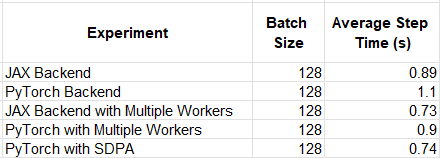
The results of our experiments are summarized in the table below. Keep in mind that the relative performance results are likely to vary greatly based on the details of the model and the runtime environment.
ViT runtime (by Author)
When using our custom attention layer, the gap between the JAX and PyTorch backends virtually disappears. This highlights how the use of a multi-backend solution could come at the expense of optimizations uniquely supported by any of the individual frameworks (in our example, PyTorch SDPA).
Keras 3 in Gemma
Gemma is a family of lightweight, open source models recently released by Google. Keras 3 plays a prominent role in the Gemma release (e.g., see here) and its multi-framework support makes Gemma automatically accessible to AI/ML developers of all persuasions — PyTorch, TensorFlow, and Jax. Please see the official documentation in KerasNLP for more details on the Gemma API offering.
# Avoid memory fragmentation on JAX backend. os.environ["XLA_PYTHON_CLIENT_MEM_FRACTION"]="1.00" os.environ["KAGGLE_USERNAME"]="chaimrand" os.environ["KAGGLE_KEY"]="29abebb28f899a81ca48bec1fb97faf1" import keras import keras_nlp keras.mixed_precision.set_global_policy('mixed_bfloat16')
import json data = [] with open("databricks-dolly-15k.jsonl") as file: for line in file: features = json.loads(line) # Filter out examples with context, to keep it simple. if features["context"]: continue # Format the entire example as a single string. template = "Instruction:n{instruction}nnResponse:n{response}" data.append(template.format(**features))
# Only use 1000 training batches, to keep it fast. data = data[:num_batches*batch_size] gemma_lm = keras_nlp.models.GemmaCausalLM.from_preset("gemma_2b_en") # Enable LoRA for the model and set the LoRA rank to 4. gemma_lm.backbone.enable_lora(rank=4)
gemma_lm.summary() # Limit the input sequence length to 512 (to control memory usage). gemma_lm.preprocessor.sequence_length = 512
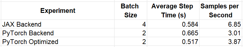
When running the script in the same GCP environment described above, we see a significant (and surprising) discrepancy between the runtime performance when using the JAX backend (6.87 samples per second) and the runtime performance when using the PyTorch backend (3.01 samples per second). This is due, in part, to the fact that the JAX backend allows for doubling the training batch size. A deep dive into the causes of this discrepancy is beyond the scope of this post.
As in our previous example, we demonstrate one way of optimizing the PyTorch runtime by prepending the following configuration of the matrix multiplication operations to the top of our script:
This simple change results in a 29% performance boost when running with the PyTorch backend. Once again, we can see the impact of applying framework-specific optimizations. The experiment results are summarized in the table below.
Gemma fine-tuning runtime (by Author)
Conclusion
Our demonstrations have indicated that sticking with the backend agnostic Keras code could imply a meaningful runtime performance penalty. In each example, we have seen how a simple, framework-specific optimization had a significant impact on the relative performance of our chosen backends. At the same time, the arguments we have discussed for multi-framework AI/ML development are rather compelling.
If you do choose to adopt Keras as a development framework, you may want to consider designing your code in a manner that includes mechanisms for applying and assessing framework-specific optimizations. You might also consider designing your development process in a way that utilizes Keras during the early stages of the project and, as the project matures, optimizes for the one backend that is revealed to be the most appropriate.
Summary
In this post we have explored the new and revised Keras 3 release. No longer an appendage to TensorFlow, Keras 3 offers the ability of framework-agnostic AI/ML model development. As we discussed, this capability has several significant advantages. However, as is often the case in the field of AI development, “there are no free lunches” — the added level of abstraction could mean a reduced level of control over the inner workings of our code which could imply slower training speed and higher costs. The best solution might be one that combines the use of Keras and its multi-framework support with dedicated mechanisms for incorporating framework-specific modifications.
Importantly, the applicability of Keras 3 to your project and the cost-best analysis of the investment required, will depend greatly on a wide variety of factors including: the target audience, the model deployment process, project timelines, and more. Please view this post as a mere introduction into your detailed exploration.
We use cookies on our website to give you the most relevant experience by remembering your preferences and repeat visits. By clicking “Accept”, you consent to the use of ALL the cookies.
This website uses cookies to improve your experience while you navigate through the website. Out of these, the cookies that are categorized as necessary are stored on your browser as they are essential for the working of basic functionalities of the website. We also use third-party cookies that help us analyze and understand how you use this website. These cookies will be stored in your browser only with your consent. You also have the option to opt-out of these cookies. But opting out of some of these cookies may affect your browsing experience.
Necessary cookies are absolutely essential for the website to function properly. These cookies ensure basic functionalities and security features of the website, anonymously.
Cookie
Duration
Description
cookielawinfo-checkbox-analytics
11 months
This cookie is set by GDPR Cookie Consent plugin. The cookie is used to store the user consent for the cookies in the category "Analytics".
cookielawinfo-checkbox-functional
11 months
The cookie is set by GDPR cookie consent to record the user consent for the cookies in the category "Functional".
cookielawinfo-checkbox-necessary
11 months
This cookie is set by GDPR Cookie Consent plugin. The cookies is used to store the user consent for the cookies in the category "Necessary".
cookielawinfo-checkbox-others
11 months
This cookie is set by GDPR Cookie Consent plugin. The cookie is used to store the user consent for the cookies in the category "Other.
cookielawinfo-checkbox-performance
11 months
This cookie is set by GDPR Cookie Consent plugin. The cookie is used to store the user consent for the cookies in the category "Performance".
viewed_cookie_policy
11 months
The cookie is set by the GDPR Cookie Consent plugin and is used to store whether or not user has consented to the use of cookies. It does not store any personal data.
Functional cookies help to perform certain functionalities like sharing the content of the website on social media platforms, collect feedbacks, and other third-party features.
Performance cookies are used to understand and analyze the key performance indexes of the website which helps in delivering a better user experience for the visitors.
Analytical cookies are used to understand how visitors interact with the website. These cookies help provide information on metrics the number of visitors, bounce rate, traffic source, etc.
Advertisement cookies are used to provide visitors with relevant ads and marketing campaigns. These cookies track visitors across websites and collect information to provide customized ads.