Originally appeared here:
How to Clean Your Data for Your Real-Life Data Science Projects
Go Here to Read this Fast! How to Clean Your Data for Your Real-Life Data Science Projects


When working on a supervised task, machine learning models can be used to predict the outcome for new samples. However, it is likely that the prediction from a new data point is incorrect. This is particularly true for a regression task where the outcome may take an infinite number of values.
In order to get a more insightful prediction, we may be interested in (or even need) a prediction interval instead of a single point. Well informed decisions should be made by taking into account uncertainty. For instance, as a property investor, I would not offer the same amount if the prediction interval is [100000–10000 ; 100000+10000] as if it is [100000–1000 ; 100000+1000] (even though the single point predictions are the same, i.e. 100000). I may trust the single prediction for the second interval but I would probably take a deep dive into the first case because the interval is quite wide, so is the profitability, and the final price may significantly differs from the single point prediction.
Before continuing, I first would like to clarify the difference between these two definitions. It was not obvious for me when I started to learn conformal prediction. Since I may not be the only one being confused, this is why I would like to give additional explanation.
ℙ([ŝ_{lb} ; ŝ_{ub}] ∋ θ) ≥ 1-α
ℙ(Y∈[ŝ_{lb} ; ŝ_{ub}]) ≥ (1-α)
Let’s consider an example to illustrate the difference. Let’s consider a n-sample of parent distribution N(μ, σ²). ŝ is the unbiased estimator of σ. <Xn> is the mean of the n-sample. I noted q the 1-α/2 quantile of the Student distribution of n-1 degree of freedom (to limit the length of the formula).
[<Xn>-q*ŝ/√(n) ; <Xn>+q*ŝ/√(n)]
[<Xn>-q*ŝ*√(1+1/n)) ; <Xn>+q*ŝ*√(1+1/n)]
Now that we have clarified these definitions, let’s come back to our goal: design insightful prediction intervals to make well informed decisions. There are many ways to design prediction intervals [2] [3]. We are going to focus on conformal predictions [4].
Conformal prediction has been introduced to generate prediction intervals with weak theoretical guarantees. It only requires that the points are exchangeable, which is weaker than i.i.d. assumption (independent and identically distributed random variables). There is no assumption on the data distribution nor on the model. By splitting the data between a training and a calibration set, it is possible to get a trained model and some non-conformity scores that we could use to build a prediction interval on a new data point (with theoretical coverage guarantee provided that the exchangeability assumption is true).
Let’s now consider an example. I would like to get some prediction intervals for house prices. I have considered the house_price dataset from OpenML [5]. I have used the library MAPIE [6] that implements conformal predictions. I have trained a model (I did not spend some time optimizing it since it is not the purpose of the post). I have displayed below the prediction points and intervals for the test set as well as the actual price.
There are 3 subplots:
– The 1st one displays the single point predictions (blue points) as well as the predictions intervals (vertical blue lines) against the true value (on abscissa). The red diagonal is the identity line. If a vertical line crosses the red line, the prediction interval does contain the actual value, otherwise it does not.
– The 2nd one displays the prediction interval widths.
– The 3rd one displays the global and local coverages. The coverage is the ratio between the number of samples falling inside the prediction intervals divided by the total number of samples. The global coverage is the ratio over all the points of the test set. The local coverages are the ratios over subsets of points of the test set. The buckets are created by means of quantiles of the actual prices.
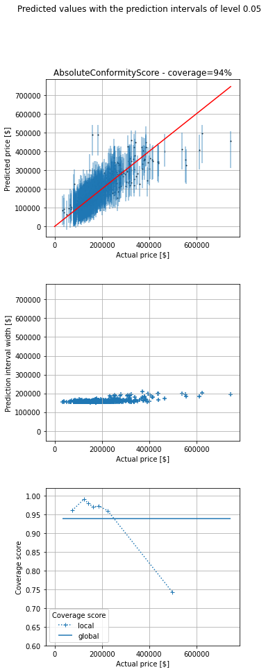
We can see that prediction width is almost the same for all the predictions. The coverage is 94%, close to the chosen value 95%. However, even though the global coverage is (close to) the desired one, if we look at (what I call) the local coverages (coverage for a subset of data points with almost the same price) we can see that coverage is bad for expensive houses (expensive regarding my dataset). Conversely, it is good for cheap ones (cheap regarding my dataset). However, the insights for cheap houses are really poor. For instance, the prediction interval may be [0 ; 180000] for a cheap house, which is not really helpful to make a decision.
Instinctively, I would like to get prediction intervals which width is proportional to the prediction value so that the prediction widths scale to the predictions. This is why I have looked at other non conformity scores, more adapted to my use case.
Even though I am not a real estate expert, I have some expectations regarding the prediction intervals. As said previously, I would like them to be, kind of, proportional to the predicted value. I would like a small prediction interval when the price is low and I expect a bigger one when the price is high.
Consequently, for this use case I am going to implement two non conformity scores that respect the conditions that a non conformity score must fulfill [7] (3.1 and Appendix C.). I have created two classes from the interface ConformityScore which requires to implement at least two methods get_signed_conformity_scores and get_estimation_distribution. get_signed_conformity_scores computes the non conformity scores from the predictions and the observed values. get_estimation_distribution computes the estimated distribution that is then used to get the prediction interval (after providing a chosen coverage). I decided to name my first non conformity score PoissonConformityScore because it is intuitively linked to the Poisson regression. When considering a Poisson regression, (Y-μ)/√μ has 0 mean and a variance of 1. Similarly, for the TweedieConformityScore class, when considering a Tweedie regression, (Y-μ)/(μ^(p/2)) has 0 mean and a variance of σ² (which is assumed to be the same for all observations). In both classes, sym=False because the non conformity scores are not expected to be symmetrical. Besides, consistency_check=False because I know that the two methods are consistent and fulfill the necessary requirements.
import numpy as np

from mapie._machine_precision import EPSILON
from mapie.conformity_scores import ConformityScore
from mapie._typing import ArrayLike, NDArray

class PoissonConformityScore(ConformityScore):
    """
    Poisson conformity score.

    The signed conformity score = (y - y_pred) / y_pred**(1/2).
    The conformity score is not symmetrical.
    y must be positive
    y_pred must be strictly positive

    This is appropriate when the confidence interval is not symmetrical and
    its range depends on the predicted values.
    """

    def __init__(
        self,
    ) -> None:
        super().__init__(sym=False, consistency_check=False, eps=EPSILON)

    def _check_observed_data(
        self,
        y: ArrayLike,
    ) -> None:
        if not self._all_positive(y):
            raise ValueError(
                f"At least one of the observed target is strictly negative "
                f"which is incompatible with {self.__class__.__name__}. "
                "All values must be positive."
            )

    def _check_predicted_data(
        self,
        y_pred: ArrayLike,
    ) -> None:
        if not self._all_strictly_positive(y_pred):
            raise ValueError(
                f"At least one of the predicted target is negative "
                f"which is incompatible with {self.__class__.__name__}. "
                "All values must be strictly positive."
            )

    @staticmethod
    def _all_positive(
        y: ArrayLike,
    ) -> bool:
        return np.all(np.greater_equal(y, 0))

    @staticmethod
    def _all_strictly_positive(
        y: ArrayLike,
    ) -> bool:
        return np.all(np.greater(y, 0))

    def get_signed_conformity_scores(
        self,
        X: ArrayLike,
        y: ArrayLike,
        y_pred: ArrayLike,
    ) -> NDArray:
        """
        Compute the signed conformity scores from the observed values
        and the predicted ones, from the following formula:
        signed conformity score = (y - y_pred) / y_pred**(1/2)
        """
        self._check_observed_data(y)
        self._check_predicted_data(y_pred)
        return np.divide(np.subtract(y, y_pred), np.power(y_pred, 1 / 2))

    def get_estimation_distribution(
        self, X: ArrayLike, y_pred: ArrayLike, conformity_scores: ArrayLike
    ) -> NDArray:
        """
        Compute samples of the estimation distribution from the predicted
        values and the conformity scores, from the following formula:
        signed conformity score = (y - y_pred) / y_pred**(1/2)
        <=> y = y_pred + y_pred**(1/2) * signed conformity score

        ``conformity_scores`` can be either the conformity scores or
        the quantile of the conformity scores.
        """
        self._check_predicted_data(y_pred)
        return np.add(y_pred, np.multiply(np.power(y_pred, 1 / 2), conformity_scores))
class TweedieConformityScore(ConformityScore):
    """
    Tweedie conformity score.

    The signed conformity score = (y - y_pred) / y_pred**(p/2).
    The conformity score is not symmetrical.
    y must be positive
    y_pred must be strictly positive

    This is appropriate when the confidence interval is not symmetrical and
    its range depends on the predicted values.
    """

    def __init__(self, p) -> None:
        self.p = p
        super().__init__(sym=False, consistency_check=False, eps=EPSILON)

    def _check_observed_data(
        self,
        y: ArrayLike,
    ) -> None:
        if not self._all_positive(y):
            raise ValueError(
                f"At least one of the observed target is strictly negative "
                f"which is incompatible with {self.__class__.__name__}. "
                "All values must be positive."
            )

    def _check_predicted_data(
        self,
        y_pred: ArrayLike,
    ) -> None:
        if not self._all_strictly_positive(y_pred):
            raise ValueError(
                f"At least one of the predicted target is negative "
                f"which is incompatible with {self.__class__.__name__}. "
                "All values must be strictly positive."
            )

    @staticmethod
    def _all_positive(
        y: ArrayLike,
    ) -> bool:
        return np.all(np.greater_equal(y, 0))

    @staticmethod
    def _all_strictly_positive(
        y: ArrayLike,
    ) -> bool:
        return np.all(np.greater(y, 0))

    def get_signed_conformity_scores(
        self,
        X: ArrayLike,
        y: ArrayLike,
        y_pred: ArrayLike,
    ) -> NDArray:
        """
        Compute the signed conformity scores from the observed values
        and the predicted ones, from the following formula:
        signed conformity score = (y - y_pred) / y_pred**(1/2)
        """
        self._check_observed_data(y)
        self._check_predicted_data(y_pred)
        return np.divide(np.subtract(y, y_pred), np.power(y_pred, self.p / 2))

    def get_estimation_distribution(
        self, X: ArrayLike, y_pred: ArrayLike, conformity_scores: ArrayLike
    ) -> NDArray:
        """
        Compute samples of the estimation distribution from the predicted
        values and the conformity scores, from the following formula:
        signed conformity score = (y - y_pred) / y_pred**(1/2)
        <=> y = y_pred + y_pred**(1/2) * signed conformity score

        ``conformity_scores`` can be either the conformity scores or
        the quantile of the conformity scores.
        """
        self._check_predicted_data(y_pred)
        return np.add(
            y_pred, np.multiply(np.power(y_pred, self.p / 2), conformity_scores)
        )
I have then taken the same example as previously. In addition to the default non conformity scores, that I named AbsoluteConformityScore in my plot, I have also considered these two additional non conformity scores.
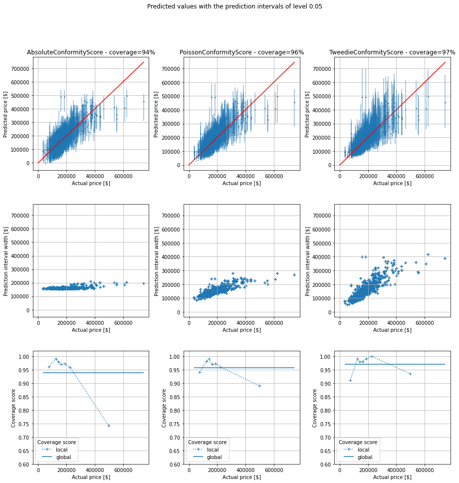
As we can see, the global coverages are all close to the chosen one, 95%. I think the small variations are due to luck during the random split between the training set and test one. However, the prediction interval widths differ significantly from an approach to another, as well as the local coverages. Once again, I am not a real estate expert, but I think the prediction intervals are more realistic for the last non conformity score (3rd column in the figure). For the new two non conformity scores, the prediction intervals are quite narrow (with a good coverage, even if slightly below 95%) for cheap houses and they are quite wide for expensive houses. This is necessary to (almost) reach the chosen coverage (95%). Our new prediction intervals from the TweedieConformityScore non conformity socre have good local coverages over the entire range of prices and are more insightful since prediction intervals are not unnecessarily wide.
Prediction intervals may be useful to make well informed decisions. Conformal prediction is a tool, among others, to build predictions intervals with theoretical coverage guarantee and only a weak assumption (data exchangeability). When considering the commonly used non conformity score, even though the global coverage is the desired one, local coverages may significantly differ from the chosen one, depending on the use case. This is why I finally considered other non conformity scores, adapted to the considered use case. I showed how to implement it in the conformal prediction library MAPIE and the benefits of doing so. An appropriate non conformity score helps to get more insightful prediction intervals (with good local coverages over the range of target values).
Adapted Prediction Intervals by Means of Conformal Predictions and a Custom Non-Conformity Score was originally published in Towards Data Science on Medium, where people are continuing the conversation by highlighting and responding to this story.
Originally appeared here:
Adapted Prediction Intervals by Means of Conformal Predictions and a Custom Non-Conformity Score
A set is a simple structure defined as a collection of distinct elements. Sets are most commonly seen in fields like mathematics or logic, but they’re also useful in programming for writing efficient code. In this article, I detail cases where sets outperform alternative data types like lists, and the underlying implementation of sets which makes them so useful to programmers.

A set is an example of a container; these are used to store several elements under one variable. When looking for a container datatype, lists (typically defined with square brackets [ ]) are the go-to choice, being used extensively in almost all programming languages. Sets bare a lot of similarity to lists, most notably as they are both dynamic, allowing their size to grow or shrink as needed. The only differences lie in that lists preserve order of elements and allow duplicates, whereas sets do neither, offering a unique advantage in certain scenarios. By knowing when to choose sets over lists, you can greatly enhance the performance of your programs and improve code readability.
In Python, sets can be declared using curly braces, or by using the set constructor.
set_a = {1, 4, 9, 16}
set_b = set([1,2,3]) #coverting list to set
empty_set = set()
A defining property of a set is that each element is distinct, or unique, so there are no repeated entries. A simple application of this could be to remove all duplicate entries in a list by converting the list into a set.
#LIST Implementation O(n^2)
def remove_duplicate_entries(list input_list):
    output_list = []
    for element in input_list:
        if element in output_list:
             output_list.append(element)
    return output_list
#SET Implementation O(n)
def remove_duplicate_entries(list input_list):
    return list(set(input_list))
Because a set is used here, the order of the list is not preserved. Use an implementation like the first one if order matters.
The next function identifies if a list contains any duplicates; the order of elements is not here important, only the occurrence of duplicates. The set implementation is much more desirable as operations on sets are typically much faster than on lists (this is explained in more detail later).
#LIST Implementation
def has_duplicates(list input_list):
    unique_elements = []
    for element in input_list:
        if element in unique_elements:
             return True
        else:
             unique_elements.append(element)
    return False
#SET Implementation
def has_duplicates(list input_list):
    return len(input_list) != len(set(input_list))
Note: In cases where a duplicate element appears early, the first implementation can outperform the second as it catches the duplicate early and returns False without checking every entry, whereas the second implementation always iterates through every element. A more optimal solution would involve a similar method to the first implementation but using a set as the unique_elements container.
def has_duplicates(list input_list) -> bool:
    unique_elements = set() #**modified here
    for element in input_list:
        if element in unique_elements:
             return True
        else:
             unique_elements.add(element)
    return False
Even if these applications seem quite crude or simplistic, there are countless uses built upon the principle of “removing duplicates” that take some creativity to see. For example, Leetcode 1832 ‘Check if the Sentence is a Pangram’- where you need to detects if all 26 letters have been used in an input sentence- can be elegantly solved using a set comprehension.
def is_pangram(str sentence) -> bool:
    present_letters = {letter for letter in sentence}
    return len(present_letters) == 26
Without sets, this problem would need to utilise nested looping which is both harder to write, and less efficient with a complexity of O(n^2).
The key to identifying cases where sets are useful is by considering:
Taking a step back, it might seem that easy duplicate removal is the only benefit of using sets. We previously discussed how sets have no order; arrays have indexed element which could simply ignored and treated like a set. It appears that arrays can do the same job as a set, if not more.
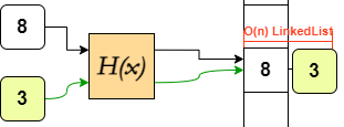
However, this simplification enforced by sets opens way to different underlying implementations. In lists, elements are assigned indices to give each element a place in the order. Sets have no need to assign indices, so they instead implement a different approach of referencing: hash mapping. These operate by (pseudo)randomly allocating addresses to elements, as opposed to storing them in a row. The allocation is governed by hashing functions, which use the element as an input to output an address.
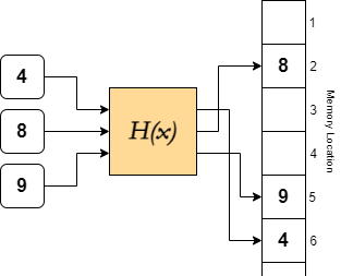
H(x) is deterministic, so the same input always gives the same output, ie. there is no RNG within the function H, so H(4) = 6 always in this case.
Running this function takes the same amount of time regardless of the size of the set, ie. hashing has O(1) time complexity. This means that the time taken to hash is independent of the size of the list, and remains at a constant, quick speed.
Because hashing is generally quick, a whole host of operations that are typically slow on large arrays can be executed very efficiently on a set.
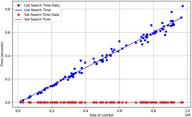
Searching for elements in an array utilises an algorithm called Linear Search, by checking each item in the list one by one. In the worst case, where the item being searched for does not exist in the list, the algorithm traverses every element of the list (O(n)). In a very large list, this process takes a long time.
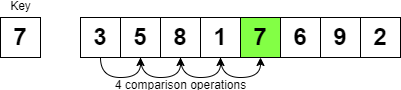
However, as hashing is O(1), Python hashes the item to be found, and either returns where it is in memory, or that it doesn’t exist- in a very small amount of time.
number_list = range(random.randint(1,000,000))
number_set = set(number_list)

#Line 1
#BEGIN TIMER
print(-1 in number_list)
#END TIMER

#Line 2
#BEGIN TIMER
print(-1 in number_set)
#END TIMER
Note: Searching using a hashmap has an amortized time complexity of O(1). This means that in the average case, it runs at constant time but technically, in the worst case, searching is O(n). However, this is extremely unlikely and comes down to the hashing implementation having a chance of collisions, which is when multiple elements in a hashmap/set are hashed to the same address.
Deleting an element from a list first involves a search to locate the element, and then removing reference to the element by clearing the address. In an array, after the O(n) time search, the index of every element following the deleted element needs to be shifted down one. This itself is another O(n) process.
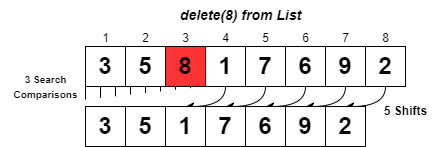
Deleting an element from a set involves the O(1) lookup, and then erasure of the memory address which is an O(1) process so deletion also operates in constant time. Sets also have more ways to delete elements, such that errors are not raised, or such that multiple elements can be removed concisely.
#LIST
numbers = [1, 3, 4, 7, 8, 11]

numbers.remove(4)
numbers.remove(5) #Raises ERROR as 5 is not in list
numbers.pop(0) #Deletes number at index 0, ie. 1

#SET
numbers = {1, 3, 4, 7, 8, 11}

numbers.remove(4)
numbers.remove(5) #Raises ERROR as 5 is not in set
numbers.discard(5) #Does not raise error if 5 is not in the set
numbers -= {1,2,3} #Performs set difference, ie. 1, 3 are discarded
Both appending to a list and adding elements to a set are constant operations; adding to a specified index in a list (.insert) however comes with the added time to shift elements around.
num_list = [1,2,3]
num_set = {1,2,3}

num_list.append(4)
num_set.add(4)

num_list += [5,6,7]
num_set += {5,6,7}
Additionally, all the mathematical operations that can be performed on sets have implementation in python also. These operations are once again time consuming to manually perform on a list, and are once again optimised using hashing.
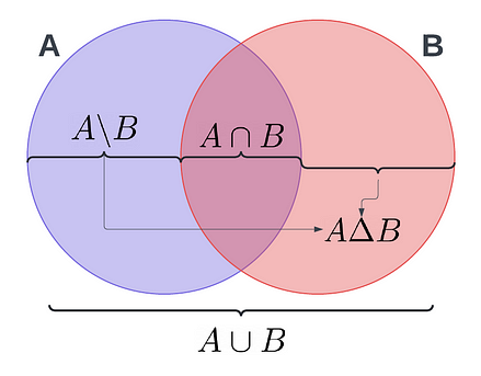
A = {1, 2, 3, 5, 8, 13}
B = {2, 3, 5, 7, 13, 17}

# A n B
AintersectB = A & B
# A U B
AunionB = A | B
# A  B
AminusB = A - B
# A U B - A n B or A Delta B
AsymmetricdiffB = A ^ B
This also includes comparison operators, namely proper and relaxed subsets and supersets. These operations once again run much faster than their list counterparts, operating in O(n) time, where n is the larger of the 2 sets.
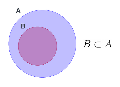
A <= B #A is a proper subset of B
A > B #A is a superset of B
A final small, but underrated feature in python is the frozen set, which is essentially a read-only or immutable set. These offer greater memory efficiency and could be useful in cases where you frequently test membership in a tuple.
The essence of using sets to boost performance is encapsulated by the principle of optimisation by reduction.
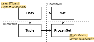
Data structures like lists have the most functionality- being indexed and dynamic- but come at the cost of comparatively lower efficiency: speed and memory-wise. Identifying which features are essential vs unused to inform what data type to use will result in code that runs faster and reads better.
All technical diagrams by author.
Why Sets are so useful in programming was originally published in Towards Data Science on Medium, where people are continuing the conversation by highlighting and responding to this story.
Originally appeared here:
Why Sets are so useful in programming
Go Here to Read this Fast! Why Sets are so useful in programming


Originally appeared here:
Using transcription confidence scores to improve slot filling in Amazon Lex

Originally appeared here:
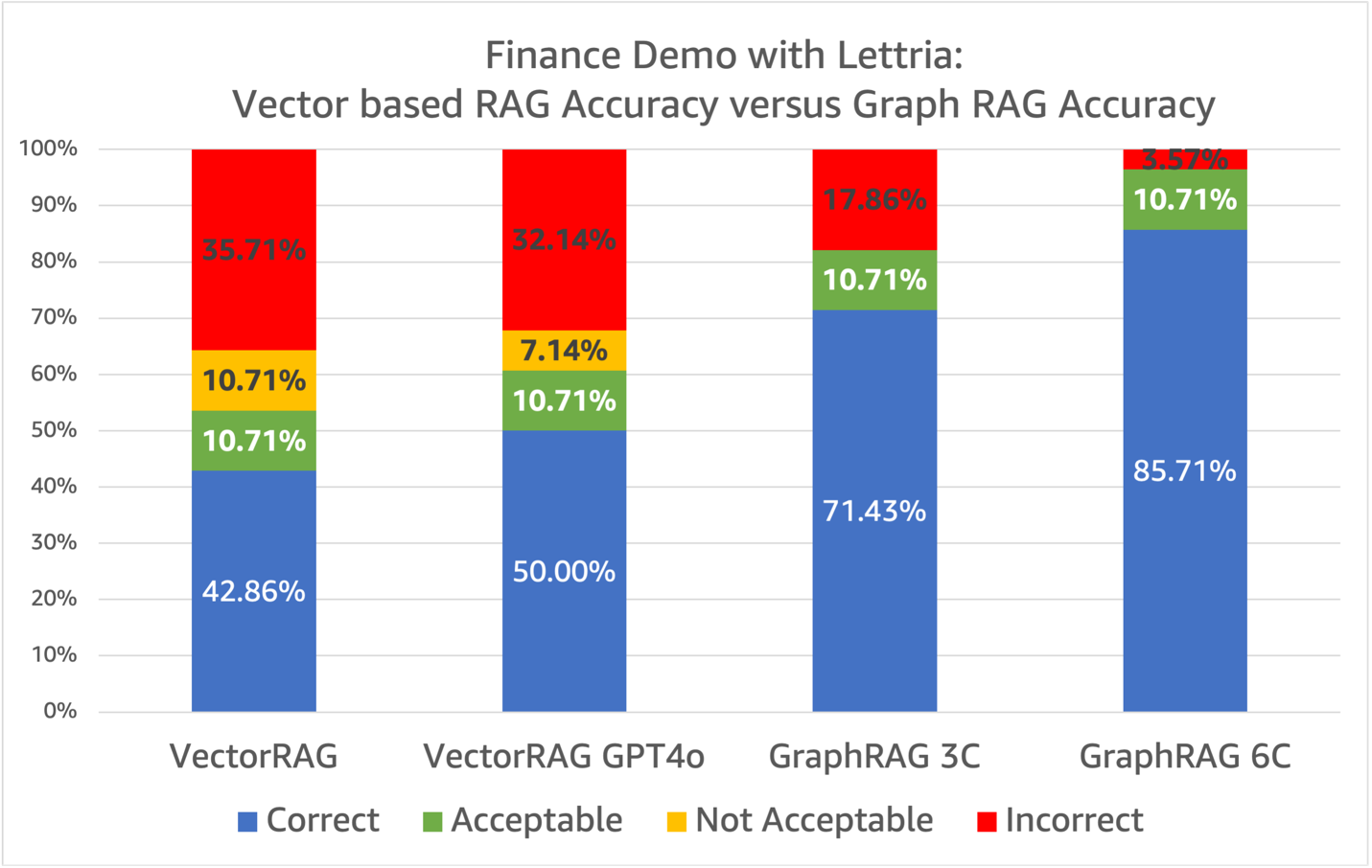
Improving Retrieval Augmented Generation accuracy with GraphRAG
Go Here to Read this Fast! Improving Retrieval Augmented Generation accuracy with GraphRAG


Understanding the exploitation-exploration trade-off with an example
Originally appeared here:
The Multi-Armed Bandit Problem—A Beginner-Friendly Guide
Go Here to Read this Fast! The Multi-Armed Bandit Problem—A Beginner-Friendly Guide
Analyze massive datasets directly in memory — faster than ever
Originally appeared here:
Handling Billions of Records in Minutes with SQL ⏱️
Go Here to Read this Fast! Handling Billions of Records in Minutes with SQL ⏱️

If you’ve worked with LLMs, you know they can sometimes hallucinate. This means they generate text that’s either nonsensical or contradicts the input data. It’s a common issue that can hurts the reliability of LLM-powered applications.
In this post, we’ll explore a few simple techniques to reduce the likelihood of hallucinations. By following these tips, you can (hopefully) improve the accuracy of your AI applications.
There are multiple types of hallucinations:
In this post, we will target all the types mentioned above.
We will list out a set of tips and tricks that work in different ways in reducing hallucinations.
Grounding is using in-domain relevant additional context in the input of the LLM when asking it to do a task. This gives the LLM the information it needs to correctly answer the question and reduces the likelihood of a hallucination. This is one the reason we use Retrieval augmented generation (RAG).
For example asking the LLM a math question OR asking it the same question while providing it with relevant sections of a math book will yield different results, with the second option being more likely to be right.
Here is an example of such implementation in one of my previous tutorials where I provide document-extracted context when asking a question:
Build a Document AI pipeline for ANY type of PDF With Gemini
Using structured outputs means forcing the LLM to output valid JSON or YAML text. This will allow you to reduce the useless ramblings and get “straight-to-the-point” answers about what you need from the LLM. It also will help with the next tips as it makes the LLM responses easier to verify.
Here is how you can do this with Gemini’s API:
import json

import google.generativeai as genai
from pydantic import BaseModel, Field

from document_ai_agents.schema_utils import prepare_schema_for_gemini


class Answer(BaseModel):
    answer: str = Field(..., description="Your Answer.")


model = genai.GenerativeModel("gemini-1.5-flash-002")

answer_schema = prepare_schema_for_gemini(Answer)


question = "List all the reasons why LLM hallucinate"

context = (
    "LLM hallucination refers to the phenomenon where large language models generate plausible-sounding but"
    " factually incorrect or nonsensical information. This can occur due to various factors, including biases"
    " in the training data, the inherent limitations of the model's understanding of the real world, and the "
    "model's tendency to prioritize fluency and coherence over accuracy."
)

messages = (
    [context]
    + [
        f"Answer this question: {question}",
    ]
    + [
        f"Use this schema for your answer: {answer_schema}",
    ]
)

response = model.generate_content(
    messages,
    generation_config={
        "response_mime_type": "application/json",
        "response_schema": answer_schema,
        "temperature": 0.0,
    },
)

response = Answer(**json.loads(response.text))

print(f"{response.answer=}")
Where “prepare_schema_for_gemini” is a utility function that prepares the schema to match Gemini’s weird requirements. You can find its definition here: code.
This code defines a Pydantic schema and sends this schema as part of the query in the field “response_schema”. This forces the LLM to follow this schema in its response and makes it easier to parse its output.
Sometimes, giving the LLM the space to work out its response, before committing to a final answer, can help produce better quality responses. This technique is called Chain-of-thoughts and is widely used as it is effective and very easy to implement.
We can also explicitly ask the LLM to answer with “N/A” if it can’t find enough context to produce a quality response. This will give it an easy way out instead of trying to respond to questions it has no answer to.
For example, lets look into this simple question and context:
Context
Thomas Jefferson (April 13 [O.S. April 2], 1743 — July 4, 1826) was an American statesman, planter, diplomat, lawyer, architect, philosopher, and Founding Father who served as the third president of the United States from 1801 to 1809.[6] He was the primary author of the Declaration of Independence. Following the American Revolutionary War and before becoming president in 1801, Jefferson was the nation’s first U.S. secretary of state under George Washington and then the nation’s second vice president under John Adams. Jefferson was a leading proponent of democracy, republicanism, and natural rights, and he produced formative documents and decisions at the state, national, and international levels. (Source: Wikipedia)
Question
What year did davis jefferson die?
A naive approach yields:
Response
answer=’1826′
Which is obviously false as Jefferson Davis is not even mentioned in the context at all. It was Thomas Jefferson that died in 1826.
If we change the schema of the response to use chain-of-thoughts to:
class AnswerChainOfThoughts(BaseModel):
    rationale: str = Field(
        ...,
        description="Justification of your answer.",
    )
    answer: str = Field(
        ..., description="Your Answer. Answer with 'N/A' if answer is not found"
    )
We are also adding more details about what we expect as output when the question is not answerable using the context “Answer with ‘N/A’ if answer is not found”
With this new approach, we get the following rationale (remember, chain-of-thought):
The provided text discusses Thomas Jefferson, not Jefferson Davis. No information about the death of Jefferson Davis is included.
And the final answer:
answer=’N/A’
Great ! But can we use a more general approach to hallucination detection?
We can, with Agents!
We will build a simple agent that implements a three-step process:
In order to implement this, we define three nodes in LangGraph. The first node will ask the question while including the context, the second node will reformulate it using the LLM and the third node will check the entailment of the statement in relation to the input context.
The first node can be defined as follows:
    def answer_question(self, state: DocumentQAState):
        logger.info(f"Responding to question '{state.question}'")
        assert (
            state.pages_as_base64_jpeg_images or state.pages_as_text
        ), "Input text or images"
        messages = (
            [
                {"mime_type": "image/jpeg", "data": base64_jpeg}
                for base64_jpeg in state.pages_as_base64_jpeg_images
            ]
            + state.pages_as_text
            + [
                f"Answer this question: {state.question}",
            ]
            + [
                f"Use this schema for your answer: {self.answer_cot_schema}",
            ]
        )

        response = self.model.generate_content(
            messages,
            generation_config={
                "response_mime_type": "application/json",
                "response_schema": self.answer_cot_schema,
                "temperature": 0.0,
            },
        )

        answer_cot = AnswerChainOfThoughts(**json.loads(response.text))

        return {"answer_cot": answer_cot}
And the second one as:
    def reformulate_answer(self, state: DocumentQAState):
        logger.info("Reformulating answer")
        if state.answer_cot.answer == "N/A":
            return

        messages = [
            {
                "role": "user",
                "parts": [
                    {
                        "text": "Reformulate this question and its answer as a single assertion."
                    },
                    {"text": f"Question: {state.question}"},
                    {"text": f"Answer: {state.answer_cot.answer}"},
                ]
                + [
                    {
                        "text": f"Use this schema for your answer: {self.declarative_answer_schema}"
                    }
                ],
            }
        ]

        response = self.model.generate_content(
            messages,
            generation_config={
                "response_mime_type": "application/json",
                "response_schema": self.declarative_answer_schema,
                "temperature": 0.0,
            },
        )

        answer_reformulation = AnswerReformulation(**json.loads(response.text))

        return {"answer_reformulation": answer_reformulation}
The third one as:
    def verify_answer(self, state: DocumentQAState):
        logger.info(f"Verifying answer '{state.answer_cot.answer}'")
        if state.answer_cot.answer == "N/A":
            return
        messages = [
            {
                "role": "user",
                "parts": [
                    {
                        "text": "Analyse the following context and the assertion and decide whether the context "
                        "entails the assertion or not."
                    },
                    {"text": f"Context: {state.answer_cot.relevant_context}"},
                    {
                        "text": f"Assertion: {state.answer_reformulation.declarative_answer}"
                    },
                    {
                        "text": f"Use this schema for your answer: {self.verification_cot_schema}. Be Factual."
                    },
                ],
            }
        ]

        response = self.model.generate_content(
            messages,
            generation_config={
                "response_mime_type": "application/json",
                "response_schema": self.verification_cot_schema,
                "temperature": 0.0,
            },
        )

        verification_cot = VerificationChainOfThoughts(**json.loads(response.text))

        return {"verification_cot": verification_cot}
Full code in https://github.com/CVxTz/document_ai_agents
Notice how each node uses its own schema for structured output and its own prompt. This is possible due to the flexibility of both Gemini’s API and LangGraph.
Lets work through this code using the same example as above ➡️
(Note: we are not using chain-of-thought on the first prompt so that the verification gets triggered for our tests.)
Context
Thomas Jefferson (April 13 [O.S. April 2], 1743 — July 4, 1826) was an American statesman, planter, diplomat, lawyer, architect, philosopher, and Founding Father who served as the third president of the United States from 1801 to 1809.[6] He was the primary author of the Declaration of Independence. Following the American Revolutionary War and before becoming president in 1801, Jefferson was the nation’s first U.S. secretary of state under George Washington and then the nation’s second vice president under John Adams. Jefferson was a leading proponent of democracy, republicanism, and natural rights, and he produced formative documents and decisions at the state, national, and international levels. (Source: Wikipedia)
Question
What year did davis jefferson die?
First node result (First answer):
relevant_context=’Thomas Jefferson (April 13 [O.S. April 2], 1743 — July 4, 1826) was an American statesman, planter, diplomat, lawyer, architect, philosopher, and Founding Father who served as the third president of the United States from 1801 to 1809.’
answer=’1826′
Second node result (Answer Reformulation):
declarative_answer=’Davis Jefferson died in 1826′
Third node result (Verification):
rationale=’The context states that Thomas Jefferson died in 1826. The assertion states that Davis Jefferson died in 1826. The context does not mention Davis Jefferson, only Thomas Jefferson.’
entailment=’No’
So the verification step rejected (No entailment between the two) the initial answer. We can now avoid returning a hallucination to the user.
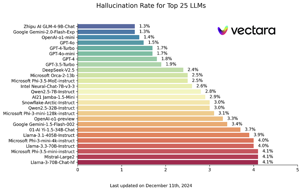
This tip is not always easy to apply due to budget or latency limitations but you should know that stronger LLMs are less prone to hallucination. So, if possible, go for a more powerful LLM for your most sensitive use cases. You can check a benchmark of hallucinations here: https://github.com/vectara/hallucination-leaderboard. We can see that the top models in this benchmark (least hallucinations) also ranks at the top of conventional NLP leader boards.
In this tutorial, we explored strategies to improve the reliability of LLM outputs by reducing the hallucination rate. The main recommendations include careful formatting and prompting to guide LLM calls and using a workflow based approach where Agents are designed to verify their own answers.
This involves multiple steps:
While all these tips can significantly improve accuracy, you should remember that no method is foolproof. There’s always a risk of rejecting valid answers if the LLM is overly conservative during verification or missing real hallucination cases. Therefore, rigorous evaluation of your specific LLM workflows is still essential.
Full code in https://github.com/CVxTz/document_ai_agents
An Agentic Approach to Reducing LLM Hallucinations was originally published in Towards Data Science on Medium, where people are continuing the conversation by highlighting and responding to this story.
Originally appeared here:
An Agentic Approach to Reducing LLM Hallucinations
Go Here to Read this Fast! An Agentic Approach to Reducing LLM Hallucinations