Stop using strings to represent paths and use pathlib instead
Originally appeared here:
Path Representation in Python

Stop using strings to represent paths and use pathlib instead
Originally appeared here:
Path Representation in Python

Simplify complex data environments for users utilizing reliable AI Agent systems towards better data-driven decision-making
Originally appeared here:
Embedding Trust into Text-to-SQL AI Agents
Go Here to Read this Fast! Embedding Trust into Text-to-SQL AI Agents
This post is a short explanation of our proposed privacy preservation technique called Privacy-PORCUPINE [1] published at Interspeech 2024 conference. The post discusses a potential privacy threat that might happen when using ordinary vector quantization in the bottleneck of DNN-based speech processing tools.
Speech is a convenient medium for interacting between humans and with technology, yet evidence demonstrates that it exposes speakers to threats to their privacy. A central issue is that, besides the linguistic content which may be private, speech contains also private side-information such as the speaker’s identity, age, state of health, ethnic background, gender, and emotions. Revealing such sensitive information to a listener may expose the speaker to threats such as price gouging, tracking, harassment, extortion, and identity theft. To protect speakers, privacy-preserving speech processing seeks to anonymize speech signals by stripping away private information that is not required for the downstream task [2].
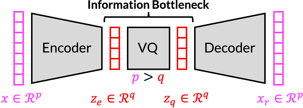
A common operating principle for privacy-preserving speech processing is to pass information through an information bottleneck that is tight enough to allow only the desired information pass through it and prevent transmission of any other private information. Such bottlenecks can be implemented for example as autoencoders, where a neural network, known as the encoder, compresses information to a bottleneck, and a second network, the decoder, reconstructs the desired output. The information rate of the bottleneck can be quantified absolutely, only if it is quantized, and quantization is thus a required component of any proof of privacy [2]. The figure below shows a vector quantized variational autoencoder (VQ-VAE) architecture, and its bottleneck.
As pointed out in the Privacy ZEBRA framework [3], we need to characterize privacy protections both in terms of average disclosure of private information (in bits) as well as worst-case disclosure (in bits). Vector quantization (VQ) [4] is a constant-bitrate quantizer in the sense that it quantizes the input with a codebook of K elements, and the indices of such a codebook can be expressed with B=log2(K) bits. This B equals to the average disclosure of private information in bits. In terms of the worst-case disclosure, it is obvious that different codebook elements are used with different frequencies (see Fig. 2.1 below). This means that a relatively smaller subset of speakers could be assigned to a particular codebook index, such that any time a speaker is assigned to that codebook index, the range of possible speakers is relatively smaller than for other codebook indices and the corresponding disclosure of private information is larger (for the speakers assigned to this particular codebook index). However, to the best of the authors’ knowledge, this disclosure has not previously been quantified nor do we have prior solutions for compensating for such an increase in disclosure. Hence, our main goal is to modify VQ such that all codebook elements have equal occurrence likelihoods to prevent private information leakage (and thus improve worst-case disclosure).
As a solution, we use here our recently proposed modification of VQ known as space-filling vector quantization (SFVQ) [5], which incorporates space-filling curves into VQ. We define the SFVQ as the linear continuation of VQ, such that subsequent codebook elements are connected with a line where inputs can be mapped to any point on that piece-wise continuous line (see Fig. 2.2). To read more about SFVQ, please see this post.
In our technique, named Privacy PORCUPINE [1], we proposed to use a codebook resampling method together with SFVQ, where a vector quantizer is resampled along the SFVQ’s curve, such that all elements of the resampled codebook have equal occurrence likelihoods (see Fig. 2.3 and 2.4).
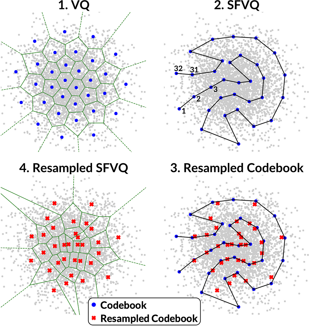
Figure 2.1 demonstrates that in areas where inputs are less likely, the Voronoi-regions are larger. Hence, such larger Voronoi-regions contain a smaller number of input samples. Similarly, small Voronoi-regions have a larger number of input samples. Such differences are due to the optimization of the codebook by minimizing the mean square error (MSE) criterion; more common inputs are quantized with a smaller error to minimize the average error. Our objective is to determine how such uneven distribution of inputs to codebook entries influences the disclosure of private information.
We measure disclosure in terms of how much the population size of possible identities for an unknown speaker is decreased with a new observation. In other words, assume that we have prior knowledge that the speaker belongs to a population of size M. If we have an observation that the speaker is quantized to an index k, we have to evaluate how many speakers L out of M will be quantized to the same index. This decrease can be quantified by the ratio of populations L/M corresponding to the disclosure of B_leak=log2(M/L) bits of information.
At the extreme, it is possible that only a single speaker may be quantized to a particular index. This means that only one speaker L=1 is quantized to the bin out of an arbitrarily large M, though in practice we can verify results only for finite M. Still, in theory, if M → ∞, then also the disclosure diverges B_leak → ∞ bits. The main objective of our proposed method is to modify vector quantization to prevent such catastrophic leaks.
After training the space-filling vector quantizer (SFVQ) [5] on the training set comprising speaker embeddings for a population of M speakers (Fig. 2.2), we map all the M embedding vectors onto the learned curve. To normalize the occurrence frequency using K codebook vectors, each codebook element has to represent M/K speaker embeddings. In other words, each Voronoi- region should encompass M/K speaker embeddings. Considering these M mapped embeddings on SFVQ’s curve, we start from the first codebook element (one end of the curve), take the first M/K mapped embeddings, and calculate the average of these vectors. We define this average vector as the new resampled codebook vector (red crosses in Fig. 2.3) representing the first chunk of M/K speaker embeddings. Then similarly, we continue until we compute all K resampled codebook vectors for all K chunks of M/K speaker embeddings.
In our experiments, we used Common Voice corpus (version 16.1) to get a large pool of speakers. We selected 10,240 speakers randomly for the test set and 79,984 speakers for the train set. To compute speaker embeddings, we used the pretrained speaker verification model of ECAPA-TDNN [6]. We trained vector quantization (VQ) and space-filling vector quantization (SFVQ) methods on the train set (of speaker embeddings) for different bitrates ranging from 4 bit to 10 bit (16 to 1024 codebook vectors).
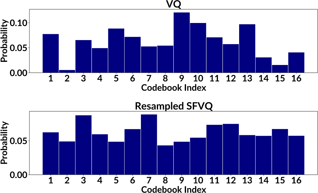
As a showcase to compare VQ and resampled SFVQ, the figure below illustrates the occurrence frequencies for VQ and resampled SFVQ, both with 4 bit of information corresponding to 16 codebook vectors. By informal visual inspection we can see that entries in the proposed method are more uniformly distributed, as desired, but to confirm results we need a proper evaluation. To compare the obtained histograms from VQ and resampled SFVQ, we used different evaluation metrics which are discussed in the next section.
Suppose we have K codebook vectors (bins) to quantize a population of M speakers. Our target is to achieve a uniform distribution of samples onto the K codebook vectors, U(1,K), such that every codebook vector is used M/K times. If we sample M integers from the uniform distribution of U(1,K), we will obtain the histogram h(k). Then, if we take the histogram of occurrences in the bins of h(k) (i.e. histogram of histogram), we will see that the new histogram follows a binomial distribution f(k) such that
where the random variable X is the occurrence in each bin, n is the number of trials (n=M), and p is the success probability for each trial which is p=1/K. After obtaining the histogram of codebook indices occurrences g(k) (Figure 3) for both VQ and resampled SFVQ methods, we compute the histogram of occurrences in the bins of g(k) denoted by f_hat(k). The binomial distribution f(k) is the theoretical optimum, to which our observation f_hat(k) should coincide. Hence, we use Kullback-Leibler (KL) divergence between f(k) and f_hat(k) to assess the distance between the observed and the ideal distributions.
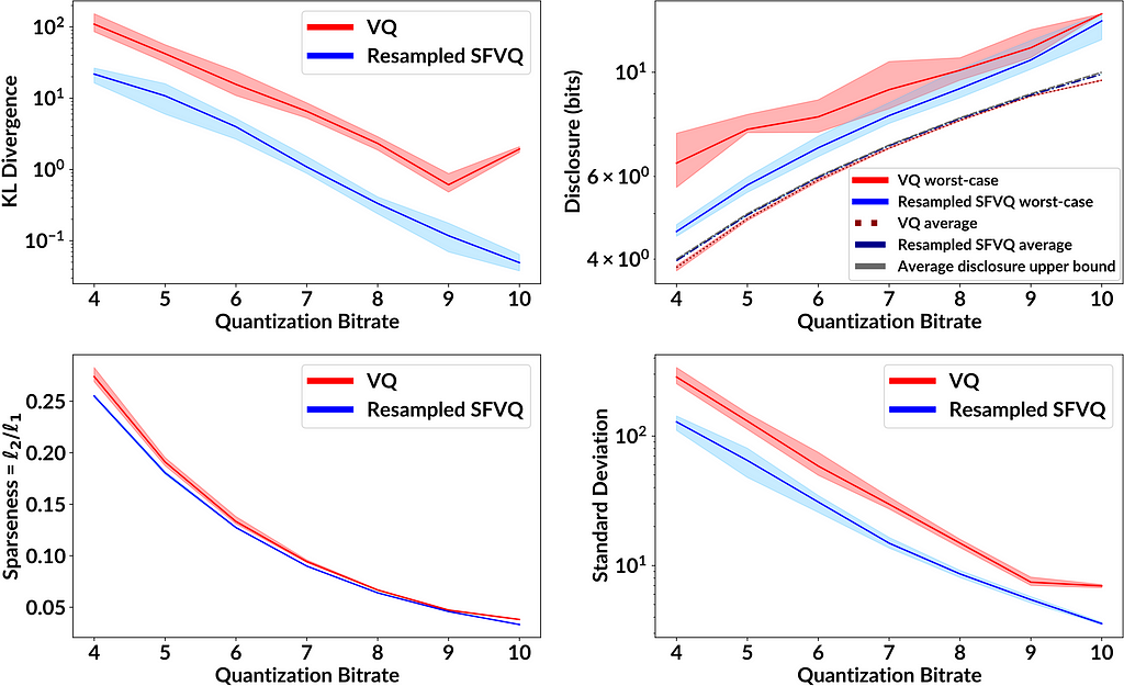
By having the histogram of occurrences g(k), we calculate the minimum of the histogram divided by the total number of samples (M=Σ g(k)) as the worst-case disclosure. We also compute the average disclosure as entropy of occurrence frequencies g(k)/M. In addition, we use a sparseness measure and standard deviation as heuristic measures of uniformity of the obtained histogram g(k). Here are the evaluation formulas:
Figure 4 shows the performance of VQ and resampled SFVQ as a function of bitrate. In each case and for all bitrates, the proposed method (blue line) is below VQ (red line), indicating that the leakage of private information is smaller for the proposed method. One important point to mention is that as expected, resampled SFVQ makes the average disclosure to be slightly higher than VQ, whereas the average disclosure for both resampled SFVQ and VQ are extremely close to the upper bound of average disclosure where the histogram of occurrence frequencies is perfectly flat.
Privacy-preserving speech processing is becoming increasingly important as the usage of speech technology is increasing. By removing superfluous private information from a speech signal by passing it through a quantized information bottleneck, we can gain provable protections for privacy. Such protections however rely on the assumption that quantization levels are used with equal frequency. Our theoretical analysis and experiments demonstrate that vector quantization, optimized with the minimum mean square (MSE) criterion, does generally not provide such uniform occurrence frequencies. In the worst case, some speakers could be uniquely identified even if the quantizer on average provides ample protection.
We proposed the resampled SFVQ method to avoid such privacy threats. The protection of privacy is thus achieved by increasing the quantization error for inputs that occur less frequently, while more common inputs gain better accuracy (see Fig. 2.4). This is in line with the theory of differential privacy [7].
We used speaker identification as an illustrative application, though the proposed method can be used in gaining a provable reduction of private information leakage for any attributes of speech. In summary, resampled SFVQ is a generic tool for privacy-preserving speech processing. It provides a method for quantifying the amount of information passing through an information bottleneck and thus forms the basis of speech processing methods with provable privacy.
The code for implementation of our proposed method and the relevant evaluations is publicly available in the following link:
GitHub – MHVali/Privacy-PORCUPINE
Special thanks to my doctoral program supervisor Prof. Tom Bäckström, who supported me and was the other contributor for this work.
[1] M.H. Vali, T. Bäckström, “Privacy PORCUPINE: Anonymization of Speaker Attributes Using Occurrence Normalization for Space-Filling Vector Quantization”, in Proceedings of Interspeech, 2024.
[2] T. Bäckström, “Privacy in speech technology”, 2024. [Online] Available at: https://arxiv.org/abs/2305.05227
[3] A. Nautsch et. al. , “The Privacy ZEBRA: Zero Evidence Biometric Recognition Assessment,” in Proceedings of Interspeech, 2020.
[4] M. H. Vali and T. Bäckström, “NSVQ: Noise Substitution in Vector Quantization for Machine Learning,” IEEE Access, 2022.
[5] M.H. Vali, T. Bäckström, “Interpretable Latent Space Using Space-Filling Curves for Phonetic Analysis in Voice Conversion”, in Proceedings of Interspeech, 2023.
[6] B. Desplanques, J. Thienpondt, and K. Demuynck, “ECAPA-TDNN: Emphasized Channel Attention, Propagation and Aggregation in TDNN Based Speaker Verification,” in Proceedings of Interspeech, 2020.
[7] C. Dwork, “Differential privacy: A survey of results,” in
International conference on theory and applications of models
of computation. Springer, 2008.
Speaker’s Privacy Protection in DNN-Based Speech Processing Tools was originally published in Towards Data Science on Medium, where people are continuing the conversation by highlighting and responding to this story.
Originally appeared here:
Speaker’s Privacy Protection in DNN-Based Speech Processing Tools
Go Here to Read this Fast! Speaker’s Privacy Protection in DNN-Based Speech Processing Tools
Steal this plug-n-play Python script to easily implement images into your chatbot’s Knowledgebase
Originally appeared here:
Don’t Limit Your RAG Knowledgebase to Just Text
Go Here to Read this Fast! Don’t Limit Your RAG Knowledgebase to Just Text

Originally appeared here:
Cohere Rerank 3 Nimble now generally available on Amazon SageMaker JumpStart

In this post we’ll identify and visualise different clusters of cancer types by analysing disease ontology as a knowledge graph. Specifically we’ll set up neo4j in a docker container, import the ontology, generate graph clusters and embeddings, before using dimension reduction to plot these clusters and derive some insights. Although we’re using `disease_ontology` as an example, the same steps can be used to explore any ontology or graph database.
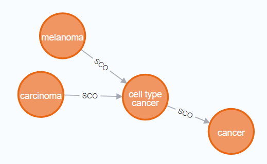
In a graph database, rather than storing data as rows (like a spreadsheet or relational database) data is stored as nodes and relationships between nodes. For example in the figure below we see that melanoma and carcinoma are SubCategories Of cell type cancer tumour (shown by the SCO relationship). With this kind of data we can clearly see that melanoma and carcinoma are related even though this is not explicitly stated in the data.
Ontologies are a formalised set of concepts and relationships between those concepts. They are much easier for computers to parse than free text and therefore easier to extract meaning from. Ontologies are widely used in biological sciences and you may find an ontology you’re interested in at https://obofoundry.org/. Here we’re focusing on the disease ontology which shows how different types of diseases relate to each other.
Neo4j is a tool for managing, querying and analysing graph databases. To make it easier to set up we’ll use a docker container.
docker run
 -it - rm
 - publish=7474:7474 - publish=7687:7687
 - env NEO4J_AUTH=neo4j/123456789
 - env NEO4J_PLUGINS='["graph-data-science","apoc","n10s"]'
 neo4j:5.17.0
In the above command the `-publish` flags set ports to let python query the database directly and let us access it through a browser. The `NEO4J_PLUGINS` argument specifies which plugins to install. Unfortunately, the windows docker image doesn’t seem to be able to handle the installation, so to follow along you’ll need to install neo4j desktop manually. Don’t worry though, the other steps should all still work for you.
While neo4j is running you can access your database by going to http://localhost:7474/ in your browser, or you can use the python driver to connect as below. Note that we’re using the port we published with our docker command above and we’re authenticating with the username and password we also defined above.
URI = "bolt://localhost:7687"
AUTH = ("neo4j", "123456789")
driver = GraphDatabase.driver(URI, auth=AUTH)
driver.verify_connectivity()
Once you have your neo4j database set up, it’s time to get some data. The neo4j plug-in n10s is built to import and handle ontologies; you can use it to embed your data into an existing ontology or to explore the ontology itself. With the cypher commands below we first set some configs to make the results cleaner, then we set up a uniqueness constraint, finally we actually import disease ontology.
CALL n10s.graphconfig.init({ handleVocabUris: "IGNORE" });
CREATE CONSTRAINT n10s_unique_uri FOR (r:Resource) REQUIRE r.uri IS UNIQUE;
CALL n10s.onto.import.fetch(http://purl.obolibrary.org/obo/doid.owl, RDF/XML);
To see how this can be done with the python driver, check out the full code here https://github.com/DAWells/do_onto/blob/main/import_ontology.py
Now that we’ve imported the ontology you can explore it by opening http://localhost:7474/ in your web browser. This lets you explore a little of your ontology manually, but we’re interested in the bigger picture so lets do some analysis. Specifically we will do Louvain clustering and generate fast random projection embeddings.
Louvain clustering is a clustering algorithm for networks like this. In short, it identifies sets of nodes that are more connected to each other than they are to the wider set of nodes; this set is then defined as a cluster. When applied to an ontology it is a fast way to identify a set of related concepts. Fast random projection on the other hand produces an embedding for each node, i.e. a numeric vector where more similar nodes have more similar vectors. With these tools we can identify which diseases are similar and quantify that similarity.
To generate embeddings and clusters we have to “project” the parts of our graph that we are interested in. Because ontologies are typically very large, this subsetting is a simple way to speed up computation and avoid memory errors. In this example we are only interested in cancers and not any other type of disease. We do this with the cypher query below; we match the node with the label “cancer” and any node that is related to this by one or more SCO or SCO_RESTRICTION relationships. Because we want to include the relationships between cancer types we have a second MATCH query that returns the connected cancer nodes and their relationships.
MATCH (cancer:Class {label:"cancer"})<-[:SCO|SCO_RESTRICTION *1..]-(n:Class)
WITH n
MATCH (n)-[:SCO|SCO_RESTRICTION]->(m:Class)
WITH gds.graph.project(
    "proj", n, m, {}, {undirectedRelationshipTypes: ['*']}
) AS g
RETURN g.graphName AS graph, g.nodeCount AS nodes, g.relationshipCount AS rels
Once we have the projection (which we have called “proj”) we can calculate the clusters and embeddings and write them back to the original graph. Finally by querying the graph we can get the new embeddings and clusters for each cancer type which we can export to a csv file.
CALL gds.fastRP.write(
  'proj',
  {embeddingDimension: 128, randomSeed: 42, writeProperty: 'embedding'}
) YIELD nodePropertiesWritten

CALL gds.louvain.write(
  "proj",
  {writeProperty: "louvain"}
) YIELD communityCount

MATCH (cancer:Class {label:"cancer"})<-[:SCO|SCO_RESTRICTION *0..]-(n)
RETURN DISTINCT
  n.label as label,
  n.embedding as embedding,
  n.louvain as louvain
Let’s have a look at some of these clusters to see which type of cancers are grouped together. After we’ve loaded the exported data into a pandas dataframe in python we can inspect individual clusters.
Cluster 2168 is a set of pancreatic cancers.
nodes[nodes.louvain == 2168]["label"].tolist()
#array(['"islet cell tumor"',
#       '"non-functioning pancreatic endocrine tumor"',
#       '"pancreatic ACTH hormone producing tumor"',
#       '"pancreatic somatostatinoma"',
#       '"pancreatic vasoactive intestinal peptide producing tumor"',
#       '"pancreatic gastrinoma"', '"pancreatic delta cell neoplasm"',
#       '"pancreatic endocrine carcinoma"',
#       '"pancreatic non-functioning delta cell tumor"'], dtype=object)
Cluster 174 is a larger group of cancers but mostly carcinomas.
nodes[nodes.louvain == 174]["label"]
#array(['"head and neck cancer"', '"glottis carcinoma"',
#       '"head and neck carcinoma"', '"squamous cell carcinoma"',
#...
#       '"pancreatic squamous cell carcinoma"',
#       '"pancreatic adenosquamous carcinoma"',
#...
#       '"mixed epithelial/mesenchymal metaplastic breast carcinoma"',
#       '"breast mucoepidermoid carcinoma"'], dtype=object)p
These are sensible groupings, based on either organ or cancer type, and will be useful for visualisation. The embeddings on the other hand are still too high dimensional to be visualised meaningfully. Fortunately, TSNE is a very useful method for dimension reduction. Here, we use TSNE to reduce the embedding from 128 dimensions down to 2, while still keeping closely related nodes close together. We can verify that this has worked by plotting these two dimensions as a scatter plot and colouring by the Louvain clusters. If these two methods agree we should see nodes clustering by colour.
from sklearn.manifold import TSNE

nodes = pd.read_csv("export.csv")
nodes['louvain'] = pd.Categorical(nodes.louvain)

embedding = nodes.embedding.apply(lambda x: ast.literal_eval(x))
embedding = embedding.tolist()
embedding = pd.DataFrame(embedding)

tsne = TSNE()
X = tsne.fit_transform(embedding)

fig, axes = plt.subplots()
axes.scatter(
    X[:,0],
    X[:,1],
    c  = cm.tab20(Normalize()(nodes['louvain'].cat.codes))
)
plt.show()
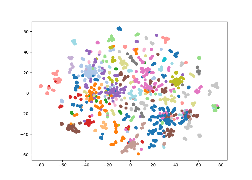
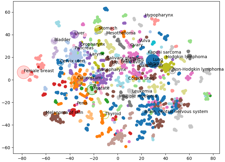
Which is exactly what we see, similar types of cancer are grouped together and visible as clusters of a single colour. Note that some nodes of a single colour are very far apart, this is because we’re having to reuse some colours as there are 29 clusters and only 20 colours. This gives us a great overview of the structure of our knowledge graph, but we can also add our own data.
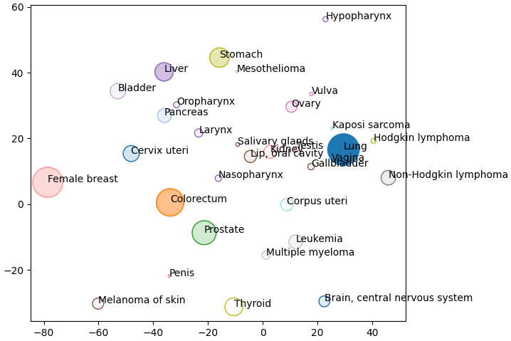
Below we plot the frequency of cancer type as node size and the mortality rate as the opacity (Bray et al 2024). I only had access to this data for a few of the cancer types so I’ve only plotted those nodes. Below we can see that liver cancer does not have an especially high incidence over all. However, incidence rates of liver cancer are much higher than other cancers within its cluster (shown in purple) like oropharynx, larynx, and nasopharynx.
Here we have used the disease ontology to group different cancers into clusters which gives us the context to compare these diseases. Hopefully this little project has shown you how to visually explore an ontology and add that information to your own data.
You can check out the full code for this project at https://github.com/DAWells/do_onto.
Bray, F., Laversanne, M., Sung, H., Ferlay, J., Siegel, R. L., Soerjomataram, I., & Jemal, A. (2024). Global cancer statistics 2022: GLOBOCAN estimates of incidence and mortality worldwide for 36 cancers in 185 countries. CA: a cancer journal for clinicians, 74(3), 229–263.
Exploring cancer types with neo4j was originally published in Towards Data Science on Medium, where people are continuing the conversation by highlighting and responding to this story.
Originally appeared here:
Exploring cancer types with neo4j
Go Here to Read this Fast! Exploring cancer types with neo4j

Working with sensitive data or within a highly regulated environment requires safe and secure cloud infrastructure for data processing. The cloud might seem like an open environment on the internet and raise security concerns. When you start your journey with Azure and don’t have enough experience with the resource configuration it is easy to make design and implementation mistakes that can impact the security and flexibility of your new data platform. In this post, I’ll describe the most important aspects of designing a cloud adaptation framework for a data platform in Azure.
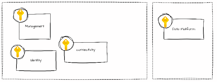
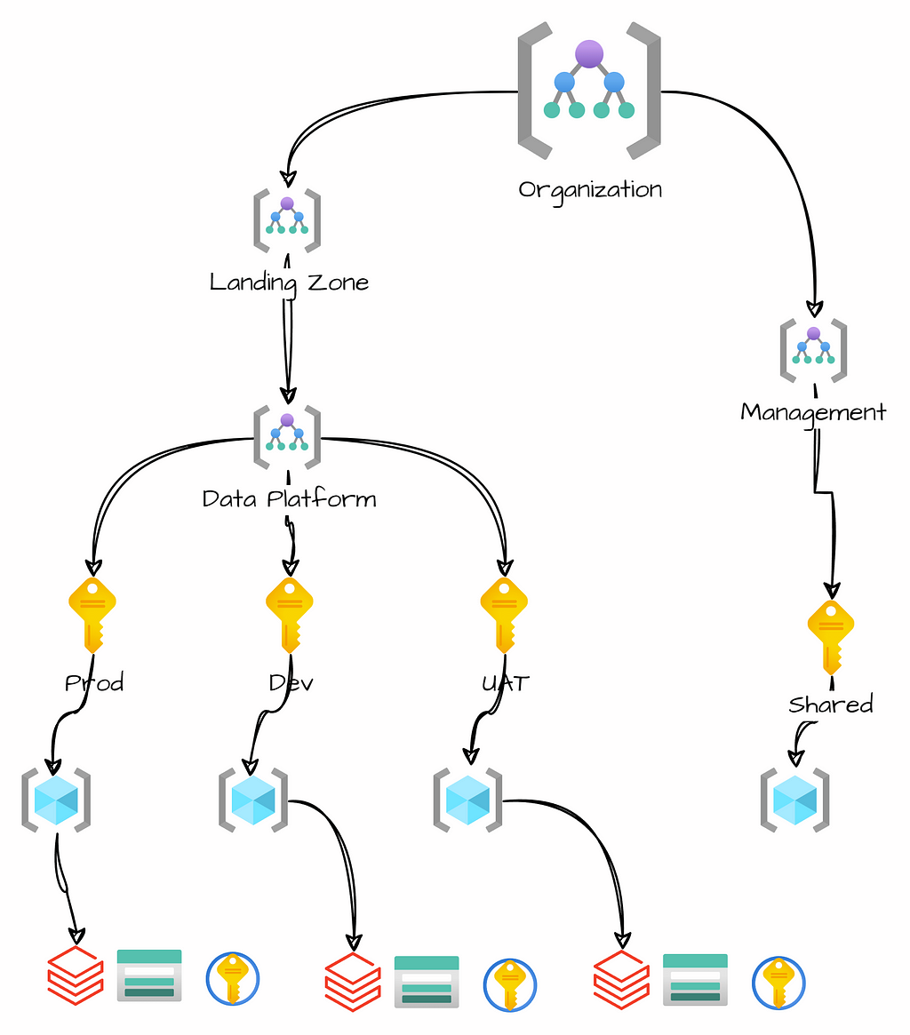
An Azure landing zone is the foundation for deploying resources in the public cloud. It contains essential elements for a robust platform. These elements include networking, identity and access management, security, governance, and compliance. By implementing a landing zone, organizations can streamline the configuration process of their infrastructure, ensuring the utilization of best practices and guidelines.
An Azure landing zone is an environment that follows key design principles to enable application migration, modernization, and development. In Azure, subscriptions are used to isolate and develop application and platform resources. These are categorized as follows:
These design principles help organizations operate successfully in a cloud environment and scale out a platform.
A data platform implementation in Azure involves a high-level architecture design where resources are selected for data ingestion, transformation, serving, and exploration. The first step may require a landing zone design. If you need a secure platform that follows best practices, starting with a landing zone is crucial. It will help you organize the resources within subscriptions and resource groups, define the network topology, and ensure connectivity with on-premises environments via VPN, while also adhering to naming conventions and standards.
Tailoring an architecture for a data platform requires a careful selection of resources. Azure provides native resources for data platforms such as Azure Synapse Analytics, Azure Databricks, Azure Data Factory, and Microsoft Fabric. The available services offer diverse ways of achieving similar objectives, allowing flexibility in your architecture selection.
For instance:
We may use Apache Spark and Python or low-code drag-and-drop tools. Various combinations of these tools can help us create the most suitable architecture depending on our skills, use cases, and capabilities.
Azure also allows you to use other components such as Snowflake or create your composition using open-source software, Virtual Machines(VM), or Kubernetes Service(AKS). We can leverage VMs or AKS to configure services for data processing, exploration, orchestration, AI, or ML.
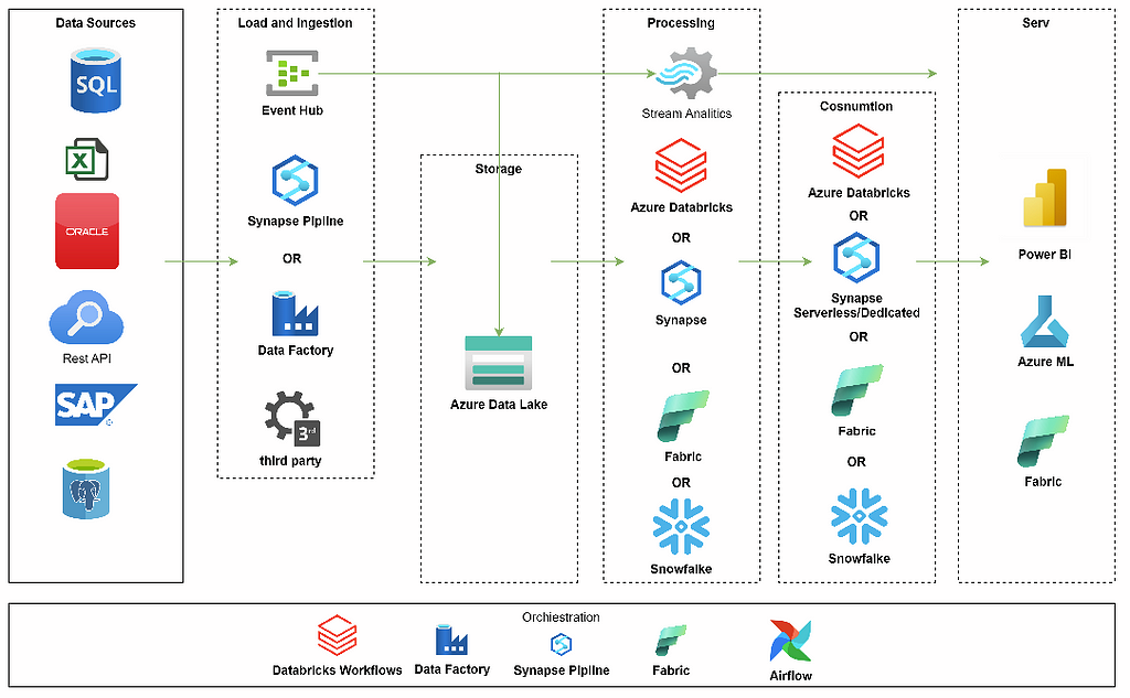
Typical Data Platform Structure
A typical Data Platform in Azure should comprise several key components:
1. Tools for data ingestion from sources into an Azure Storage Account. Azure offers services like Azure Data Factory, Azure Synapse Pipelines, or Microsoft Fabric. We can use these tools to collect data from sources.
2. Data Warehouse, Data Lake, or Data Lakehouse: Depending on your architecture preferences, we can select different services to store data and a business model.
3. To orchestrate data processing in Azure we have Azure Data Factory, Azure Synapse Pipelines, Airflow, or Databricks Workflows.
4. Data transformation in Azure can be handled by various services.
An important aspect of platform design is planning the segmentation of subscriptions and resource groups based on business units and the software development lifecycle. It’s possible to use separate subscriptions for production and non-production environments. With this distinction, we can achieve a more flexible security model, separate policies for production and test environments, and avoid quota limitations.
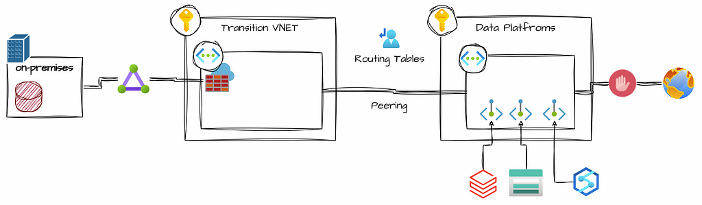
A virtual network is similar to a traditional network that operates in your data center. Azure Virtual Networks(VNet) provides a foundational layer of security for your platform, disabling public endpoints for resources will significantly reduce the risk of data leaks in the event of lost keys or passwords. Without public endpoints, data stored in Azure Storage Accounts is only accessible when connected to your VNet.
The connectivity with an on-premises network supports a direct connection between Azure resources and on-premises data sources. Depending on the type of connection, the communication traffic may go through an encrypted tunnel over the internet or a private connection.
To improve security within a Virtual Network, you can use Network Security Groups(NSGs) and Firewalls to manage inbound and outbound traffic rules. These rules allow you to filter traffic based on IP addresses, ports, and protocols. Moreover, Azure enables routing traffic between subnets, virtual and on-premise networks, and the Internet. Using custom Route Tables makes it possible to control where traffic is routed.
A naming convention establishes a standardization for the names of platform resources, making them more self-descriptive and easier to manage. This standardization helps in navigating through different resources and filtering them in Azure Portal. A well-defined naming convention allows you to quickly identify a resource’s type, purpose, environment, and Azure region. This consistency can be beneficial in your CI/CD processes, as predictable names are easier to parametrize.
Considering the naming convention, you should account for the information you want to capture. The standard should be easy to follow, consistent, and practical. It’s worth including elements like the organization, business unit or project, resource type, environment, region, and instance number. You should also consider the scope of resources to ensure names are unique within their context. For certain resources, like storage accounts, names must be unique globally.
For example, a Databricks Workspace might be named using the following format:
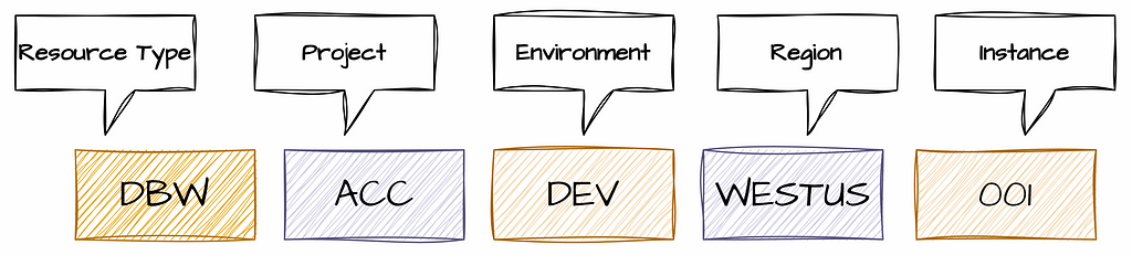
Example Abbreviations:
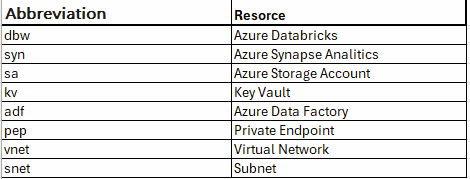
A comprehensive naming convention typically includes the following format:
Implementing infrastructure through the Azure Portal may appear straightforward, but it often involves numerous detailed steps for each resource. The highly secured infrastructure will require resource configuration, networking, private endpoints, DNS zones, etc. Resources like Azure Synapse or Databricks require additional internal configuration, such as setting up Unity Catalog, managing secret scopes, and configuring security settings (users, groups, etc.).
Once you finish with the test environment, you‘ll need to replicate the same configuration across QA, and production environments. This is where it’s easy to make mistakes. To minimize potential errors that could impact development quality, it‘s recommended to use an Infrastructure as a Code (IasC) approach for infrastructure development. IasC allows you to create cloud infrastructure as code in Terraform or Biceps, enabling you to deploy multiple environments with consistent configurations.
In my cloud projects, I use accelerators to quickly initiate new infrastructure setups. Microsoft also provides accelerators that can be used. Storing an infrastructure as a code in a repository offers additional benefits, such as version control, tracking changes, conducting code reviews, and integrating with DevOps pipelines to manage and promote changes across environments.
If your data platform doesn’t handle sensitive information and you don’t need a highly secured data platform, you can create a simpler setup with public internet access without Virtual Networks(VNet), VPNs, etc. However, in a highly regulated area, a completely different implementation plan is required. This plan will involve collaboration with various teams within your organization — such as DevOps, Platform, and Networking teams — or even external resources.
You’ll need to establish a secure network infrastructure, resources, and security. Only when the infrastructure is ready you can start activities tied to data processing development.
If you found this article insightful, I invite you to express your appreciation by clicking the ‘clap’ button or liking it on LinkedIn. Your support is greatly valued. For any questions or advice, feel free to contact me on LinkedIn.
Adapting the Azure Landing Zone for a Data Platform in the Cloud was originally published in Towards Data Science on Medium, where people are continuing the conversation by highlighting and responding to this story.
Originally appeared here:
Adapting the Azure Landing Zone for a Data Platform in the Cloud
Go Here to Read this Fast! Adapting the Azure Landing Zone for a Data Platform in the Cloud