Traditional monitoring no longer meets the needs of complex data organizations. Instead of relying on reactive systems to identify known issues, data engineers must create interactive observability frameworks that help them quickly find any type of anomaly.
While observability can encompass many different practices, in this article, I’ll share a high-level overview and practical tips from our experience building an observability framework in our organization using open-source tools.
So, how to build infrastructure that has good data health visibility and ensures data quality?
What is data observability?
Overall, observability defines how much you can tell about an internal system from its external outputs. The term was first defined in 1960 by Hungarian-American engineer Rudolf E. Kálmán, who discussed observability in mathematical control systems.
Over the years, the concept has been adapted to various fields, including data engineering. Here, it addresses the issue of data quality and being able to track where the data was gathered and how it was transformed.
Data observability means ensuring that data in all pipelines and systems is integral and of high quality. This is done by monitoring and managing real-time data to troubleshoot quality concerns. Observability assures clarity, which allows action before the problem spreads.
What is a data observability framework?
Data observability framework is a process of monitoring and validating data integrity and quality within an institution. It helps to proactively ensure data quality and integrity.
The framework must be based on five mandatory aspects, as defined by IBM:
Freshness. Outdated data, if any, must be found and removed.
Distribution. Expected data values must be recorded to help identify outliers and unreliable data.
Volume. The number of expected values must be tracked to ensure data is complete.
Schema. Changes to data tables and organization must be monitored to help find broken data.
Lineage. Collecting metadata and mapping the sources is a must to aid troubleshooting.
These five principles ensure that data observability frameworks help maintain and increase data quality. You can achieve these by implementing the following data observability methods.
How to add observability practices into the data pipeline
Only high-quality data collected from reputable sources will provide precise insights. As the saying goes: garbage in, garbage out. You cannot expect to extract any actual knowledge from poorly organized datasets.
As a senior data analyst at public data provider Coresignal, I constantly seek to find new ways to improve data quality. While it’s quite a complex goal to achieve in the dynamic tech landscape, many paths lead to it. Good data observability plays an important role here.
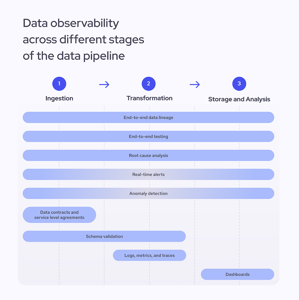
So, how do we ensure the quality of data? It all comes down to adding better observability methods into each data pipeline stage — from ingestion and transformation to storage and analysis. Some of these methods will work across the entire pipeline while others will be relevant in only one stage of it. Let’s take a look:
Data observability across different stages of the data pipeline. Source: Jurgita Motus
First off, we have to consider five items that cover the entire pipeline:
End-to-end data lineage. Tracking lineage lets you quickly access database history and follow your data from the original source to the final output. By understanding the structure and its relationships, you will have less trouble finding inconsistencies before they become problems.
End-to-end testing. A validation process that checks data integrity and quality at each data pipeline stage helps engineers determine if the pipeline functions correctly and spot any untypical behaviors.
Root cause analysis. If issues emerge at any stage of the pipeline, engineers must be able to pinpoint the source precisely and find a quick solution.
Real-time alerts. One of the most important observability goals is to quickly spot emerging issues. Time is of the essence when flagging abnormal behaviors, so any data observability framework has to be able to send alerts in real time. This is especially important for the data ingestion as well as storage and analysis phases.
Anomaly detection. Issues such as missing data or low performance can happen anywhere across the data pipeline. Anomaly detection is an advanced observability method that is likely to be implemented later in the process. In most cases, machine learning algorithms will be required to detect unusual patterns in your data and logs.
Then, we have five other items that will be more relevant in one data pipeline stage than the other:
Service level agreements (SLAs). SLAs help set standards for the client and the supplier and define the data quality, integrity, and general responsibilities. SLA thresholds can also help when setting up an alert system, and typically, they will be signed before or during the ingestion phase.
Data contracts. These agreements define how data is structured before it enters other systems. They act as a set of rules that clarify what level of freshness and quality you can expect and will usually be negotiated before the ingestion phase.
Schema validation. It guarantees consistent data structures and ensures compatibility with downstream systems. Engineers usually validate the schema during the ingestion or processing stages.
Logs, metrics, and traces. While essential for monitoring performance, collecting and easily accessing this crucial information will become a helpful tool in a crisis — it allows one to find the root cause of a problem faster.
Data quality dashboards. Dashboards help monitor the overall health of the data pipeline and have a high-level view of possible problems. They ensure that the data gathered using other observability methods is presented clearly and in real time.
Finally, data observability cannot be implemented without adding self-evaluation to the framework, so constant auditing and reviewing of the system is a must for any organization.
Next, let’s discuss the tools you might want to try to make your work easier.
Data observability platforms and what can you do with them
So, which tools should you consider if you are beginning to build a data observability framework in your organization? While there are many options out there, in my experience, your best bet would be to start out with the following tools.
As we were building our data infrastructure, we focused on making the most out of open source platforms. The tools listed below ensure transparency and scalability while working with large amounts of data. While most of them have other purposes than data observability, combined, they provide a great way to ensure visibility into the data pipeline.
Here is a list of five necessary platforms that I would recommend to check out:
Prometheus and Grafana platforms complement each other and help engineers collect and visualize large amounts of data in real time. Prometheus, an open-source monitoring system, is perfect for data storage and observation, while the observability platform Grafana helpstrack new trends through an easy-to-navigate visual dashboard.
Apache Iceberg table format provides an overview of database metadata, including tracking statistics about table columns. Tracking metadata helps to better understand the entire database without unnecessarily processing it. It’s not exactly an observability platform, but its functionalities allow engineers to get better visibility into their data.
Apache Superset is another open-source data exploration and visualization tool that can help to present huge amounts of data, build dashboards, and generate alerts.
Great Expectations is a Python package that helps test and validate data. For instance, it can scan a sample dataset using predefined rules and create data quality conditions that are later used for the entire dataset. Our teams use Great Expectations torun quality tests on new datasets.
Dagster data pipeline orchestration tool can help ensure data lineage and run asset checks. While it was not created as a data observability platform, it provides visibility using your existing data engineering tools and table formats. The tool aids in figuring out the root causes of data anomalies. The paid version of the platform also contains AI-generated insights. This application provides self-service observability and comes with an in-built asset catalog for tracking data assets.
Keep in mind that these are just some of the many options available. Make sure to do your research and find the tools that make sense for your organization.
What happens if you ignore the data observability principles
Once a problem arises, organizations usually rely on an engineer’s intuition to find the root cause of the problem. As software engineer Charity Majors vividly explains in her recollection of her time at MBaaS platform Parse, most traditional monitoring is powered by engineers who have been at the company the longest and can quickly guess their system’s issues. This makes senior engineers irreplaceable and creates additional issues, such as high rates of burnout.
Using data observability tools eliminates guesswork from troubleshooting, minimizes the downtime, and enhances trust. Without data observability tools, you can expect high downtime, data quality issues, and slow reaction times to emerging issues. As a result, these problems might quickly lead to loss of revenue, customers, or even damage brand reputation.
Data observability is vital for enterprise-level companies that handle gargantuan amounts of information and must guarantee its quality and integrity without interruptions.
What’s next for data observability?
Data observability is a must for every organization, especially companies that work with data collection and storage. Once all the tools are set in place, it’s possible to start using advanced methods to optimize the process.
Machine learning, especially large language models (LLMs), is the obvious solution here. They can help to quickly scan the database, flag anomalies, and help to improve the overall data quality by spotting duplicates or adding new enriched fields. At the same time, these algorithms can help keep track of the changes in the schema and logs, improving the data consistency and improving data lineage.
However, it is crucial to pick the right time to implement your AI initiatives. Enhancing your observability capabilities requires resources, time, and investment. Before starting to use custom LLMs, you should carefully consider whether this would truly benefit your organization. Sometimes, it might be more efficient to stick to the standard open-source data observability tools listed above, which are already effective in getting the job done.
A powerful yet under-the-radar method for data summarization and explainable AI
Despite being a powerful tool for data summarization, the MMD-Critic method has a surprising lack of both usage and “coverage”. Perhaps this is because simpler and more established methods for data summarization exist (e.g. K-medoids, see [1] or, more simply, the Wikipedia page), or perhaps this is because no Python package for the method existed (before now). Regardless, the results presented in the original paper [2] warrant more use than MMD-Critic has currently. As such, I’ll explain the MMD-Critic method here with as much clarity as possible. I’ve also published an open-source Python package with an implementation of the technique so you can use it easily.
Prototypes and Criticisms
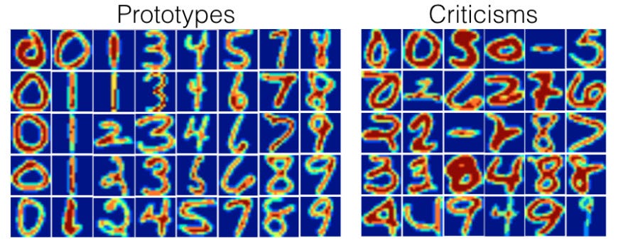
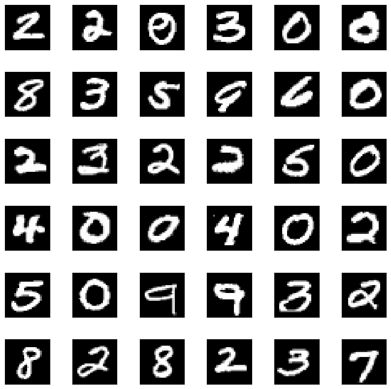
Before jumping into the MMD-Critic method itself, it’s worth discussing what exactly we’re trying to accomplish. Ultimately, we wish to take a dataset and find examples that are representative of the data (prototypes), as well as edge-case examples that may confound our machine learning models (criticisms).
Prototypes and criticisms for the MNIST dataset, taken from [2].
There are many reasons why this may be useful:
We can get a very nice summarized view of our dataset by seeing both stereotypical and atypical examples
We can test models on the criticisms to see how they handle edge cases (this is, for obvious reasons, very important)
Though perhaps not as useful, we can use prototypes to create a naturally explainable K-means-esque algorithm wherein the closest prototype to the new data point is used to label it. Then explanations are simple since we just show the user the most similar data point.
More
You can see section 6.3 in this book for more info on the applications of this (and for a decent explanation of MMD-Critic as well), but it suffices to say that finding these examples is useful for a wide variety of reasons. MMD-Critic allows us to do this.
Maximal Mean Discrepancy
I unfortunately cannot claim to have a hyper-rigorous understanding of Maximal Mean Discrepancy (MMD), as such an understanding would require a strong background in functional analysis. If you have such a background, you can find the paper that introduced the measure here.
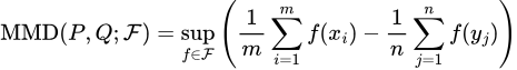
In simple terms though, MMD is a way to determine the difference between two probability distributions. Formally, for two probability distributions P and Q, we define the MMD of the two as
The formula for the MMD of two distributions P, Q
Here, F is any function space — that is, any set of functions with the same domain and codomain. Note also that the notation x~P means that we are treating x as if it’s a random variable drawn from the distribution P — that is, x is described byP. This formula thus finds the highest difference in the expected values of X and Y when they are transformed by some function from our space F.
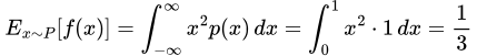
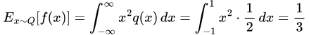
This may be a little hard to wrap your head around, but here’s an example. Suppose that X is Uniform(0, 1) (i.e. a distribution that is equivalent to picking a random number from 0 to 1), and Y is Uniform(-1, 1) . Let’s also let F be a fairly simple family containing three functions — f(x) = 0, f(x) = x, and f(x) = x². Iterating over each function in our space, we get:
In the f(x)= 0 case, E[f(x)] when x ~ P is 0 since no matter what x we choose, f(x) will be 0. The same holds for when x ~ Q. Thus, we get a mean discrepancy of 0
In the f(x) = x case, we have E[f(x)] = 0.5 for the P case and 0 for the Q case, so our mean discrepancy is 0.5
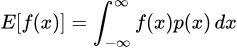
In the f(x) = x² case, we note that
Formula for the expected value of a random variable x transformed by a function f
thus in the P case, we get
Expected value of f(x) under the distribution P
and in the Q case, we get
Expected value of f(x) under the distribution Q
thus our discrepancy in this case is also 0. The supremum over our function space is thus 0.5, so that’s our MMD.
You may now notice a few problems with our MMD. It seems highly dependent on our choice of function space and also appears highly expensive (or even impossible) to compute for a large or infinite function space. Not only that, but it also requires us to know our distributions P and Q, which is not realistic.
The latter problem is easily solvable, as we can rewrite our MMD metric to use estimates of P and Q based on our dataset:
MMD using estimates of P and Q
Here, our x’s are our samples from the dataset drawing from P, and the y’s are the samples drawn from Q.
The first two problems are solvable with a bit of extra math. Without going into too much detail, it turns out that if F is something called a Reproducing Kernel Hilbert Space (RKHS), we know what function is going to give us our MMD in advance. Namely, it’s the following function, called the witness function:
Our optimal f(x) in an RKHS
where k is the kernel (inner product) associated with the RKHS¹. Intuitively, this function “witnesses” the discrepancy between P and Q at the point x.
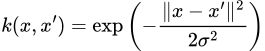
We thus only need to choose a sufficiently expressive RKHS/kernel — usually, the RBF kernel is used which has the kernel function
The RBF kernel, where sigma is a hyperparameter
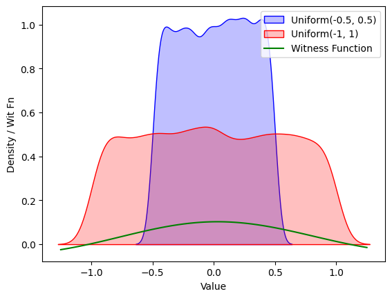
This generally gets fairly intuitive results. Here, for instance, is the plot of the witness function with the RBF kernel when estimated (in the same way as mentioned before — that is, replacing expectations with a sum) on two datasets drawn from Uniform(-0.5, 0.5) and Uniform(-1, 1) :
Values of the witness function at different points for two uniform distributions
The code for generating the above graph is here:
import numpy as np import matplotlib.pyplot as plt import seaborn as sns
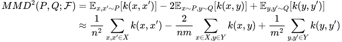
The idea behind MMD-Critic is now fairly simple — if we want to find k prototypes, we need to find the set of prototypes that best matches the distribution of the original dataset given by their squared MMD. In other words, we wish to find a subset P of cardinality k of our dataset that minimizes MMD²(F, X, P). Without going into too much detail about why, the square MMD is given by
The square MMD metric, with X ~ P, Y ~ Q, and k the kernel for our RKHS F
After finding these prototypes, we then select the points where the hypothetical distribution of our prototypes is most different from our dataset distribution as criticisms. As we’ve seen before, the difference between two distributions at a point can be measured by our witness function, so we just find points that maximize its absolute value in the context of X and P. In other words, we define our criticism “score” as
The “score” for a criticism c
Or, in the more usable approximate form,
The approximated S(c) for a criticism c
Then, to find our desired amount of criticisms, say m of them, we simply wish to find the set C of size m that maximizes
To promote picking more varied criticisms, the paper also suggests adding a regularizer term that encourages selected criticisms to be as far apart as possible. The suggested regularizer in the paper is the log determinant regularizer, though this is not required. I won’t go into much detail here since it’s not critical, but the paper suggests reading [6]².
We can thus implement an extremely naive MMD-Critic without criticism regularization as follows (do NOT use this):
import math import itertools
def euc_distance(p1, p2): return math.sqrt(sum((x - y) ** 2 for x, y in zip(p1, p2)))
def select_protos(X, n, sigma=0.5): min_score, min_sub = math.inf, None for subset in itertools.combinations(X, n): new_mmd = mmd_sq(X, subset, sigma) if new_mmd < min_score: min_score = new_mmd min_sub = subset return min_sub
def criticism_score(criticism, prototypes, X, sigma=0.5): return abs(1/len(X) * sum([rbf(criticism, x, sigma) for x in X]) - 1/len(prototypes) * sum([rbf(criticism, p, sigma) for p in prototypes]))
def select_criticisms(X, P, n, sigma=0.5): candidates = [c for c in X if c not in P] max_score, crits = -math.inf, [] for subset in itertools.combinations(candidates, n): new_score = sum([criticism_score(c, P, X, sigma) for c in subset]) if new_score > max_score: max_score = new_score crits = subset
return crits
Optimizing MMD-Critic
The above implementation is so impractical that, when I ran it, I failed to find 5 prototypes in a dataset with 25 points in a reasonable time. This is because our MMD calculation is O(max(|X|, |Y|)²), and iterating over every length-n subset is O(C(|X|, n)) (where C is the choose function), which gives us a horrendous runtime complexity.
Disregarding using more efficient computation methods (e.g. using pure numpy/numexpr/matrix calculations instead of loops/whatever) and caching repeated calculations, there are a few optimizations we can make on the theoretical level. Firstly, the most obvious slowdown we have is looping over the C(|X|, n) subsets in our prototype and criticism methods. Instead of that, we can use an approximation that loops n times, greedily selecting the best prototype each time. This allows us to change our prototype selection code to
def select_protos(X, n, sigma=0.5):
  protos = []
  for _ in range(n):
    min_score, min_proto = math.inf, None
    for cand in X:
      if cand in protos:
        continue
      new_score = mmd_sq(X, protos + [cand], sigma)
      if new_score < min_score:
        min_score = new_score
        min_proto = cand
    protos.append(min_proto)
  return protos
and similar for the criticisms.
There’s one other important lemma that makes this problem much more optimizable. It turns out that by changing our prototype selection into a minimization problem and adding a regularization term to the cost, we can compute the cost function very efficiently with matrix operations. I won’t go into much detail here, but you can check out the original paper for details.
Playing With the MMD-Critic Package
Now that we understand the MMD-Critic method, we can finally play with it! You can install it by running
pip install mmd-critic
The implementation in the package itself is much faster than the one presented here, so don’t worry.
We can run a fairly simple example using blobs as such:
from sklearn.datasets import make_blobs from mmd_critic import MMDCritic from mmd_critic.kernels import RBFKernel
n_samples = 50 # Total number of samples centers = 4 # Number of clusters cluster_std = 1 # Standard deviation of the clusters
# MMD critic with the kernel used for the prototypes being an RBF with sigma=1, # for the criticisms one with sigma=0.025 critic = MMDCritic(X, RBFKernel(1), RBFKernel(0.025)) protos, _ = critic.select_prototypes(centers) criticisms, _ = critic.select_criticisms(10, protos)
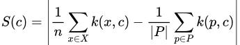
Then plotting the points and criticisms gets us
Plotting the found prototypes (green) and criticisms (red)
You’ll notice that I provided the option to use a separate kernel for prototype and criticism selection. This is because I’ve found that results for criticisms especially can be extremely sensitive to the sigma hyperparameter. This is an unfortunate limitation of the MMD Critic method and kernel methods in general. Overall, I’ve found good results using a large sigma for prototypes and a smaller one for criticisms.
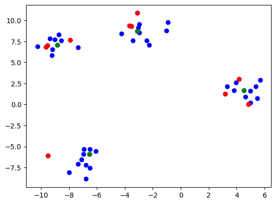
We can also, of course, use a more complicated dataset. Here, for instance, is the method used on MNIST³:
from sklearn.datasets import fetch_openml import numpy as np from mmd_critic import MMDCritic from mmd_critic.kernels import RBFKernel
Prototypes found by MMD critic for MNIST. MNIST is free for commercial use under the GPL-3.0 License.
and criticisms
Criticisms found by the MMD Critic method
Pretty neat, huh?
Conclusions
And that’s about it for the MMD-Critic method. It is quite simple at the core, and it is nice to use save for having to fiddle with the Sigma hyperparameter. I hope that the newly released Python package gives it more use.
Please contact [email protected] for any inquiries. All images by author unless stated otherwise.
Footnotes
[1] You may be familiar with RKHSs and kernels if you’ve ever studied SVMs and the kernel trick — the kernels used there are just inner products in some RKHS. The most common is the RBF kernel, for which the associated RKHS of functions is an infinite-dimensional set of smooth functions.
[2] I have not read this source beyond a brief skim. It seems mostly irrelevant, and the log determinant regularizer is fairly simple to implement. If you want to read it though, go for it.
[3] For legal reasons, you can find a repository with the MNIST dataset here. It is free for commercial use under the GPL-3.0 License.
Diffusers and Quanto giving hope to the GPU-challenged
Generated locally by PixArt-Σ with less than 8Gb of VRam
Image generation tools are hotter than ever, and they’ve never been more powerful. Models like PixArt Sigma and Flux.1 are leading the charge, thanks to their open weight models and permissive licenses. This setup allows for creative tinkering, including training LoRAs without sharing data outside your computer.
However, working with these models can be challenging if you’re using older or less VRAM-rich GPUs. Typically, there’s a trade-off between quality, speed, and VRAM usage. In this blog post, we’ll focus on optimizing for speed and lower VRAM usage while maintaining as much quality as possible. This approach works exceptionally well for PixArt due to its smaller size, but results might vary with Flux.1. I’ll share some alternative solutions for Flux.1 at the end of this post.
Both PixArt Sigma and Flux.1 are transformer-based, which means they benefit from the same quantization techniques used by large language models (LLMs). Quantization involves compressing the model’s components to use less memory. It allows you to keep all model components in GPU VRAM simultaneously, leading to faster generation speeds compared to methods that move weights between the GPU and CPU, which can slow things down.
Let’s dive into the setup!
Setting Up Your Local Environment
First, ensure you have Nvidia drivers and Anaconda installed.
Next, create a python environment and install all the main requirements:
Understanding the Script: Here are the major steps of the implementation
Import Necessary Libraries: We import libraries for quantization, model loading, and GPU handling.
Load the Model: We load the PixArt Sigma model in half-precision (float16) to CPU first.
Quantize the Model: We apply quantization to the transformer and text encoder components of the model. Here we apply different levels of quantizations: The Text encoder part is quantized at qint4 given that it is quite large. The vision part, if quantized at qint8, would make the full pipeline use up 7.5 G VRAM, if not quantized at all would use around 8.5 G VRAM.
Move to GPU: We move the pipeline to the GPU .to(“cuda”)for faster processing.
Generate Images: We use the pipe to generate images based on a given prompt and save the output.
Running the Script
Save the script and run it in your environment. You should see an image generated based on the prompt “Cyberpunk cityscape, small black crow, neon lights, dark alleys, skyscrapers, futuristic, vibrant colors, high contrast, highly detailed” saved as sigma_1.png. Generation takes 6 seconds on a RTX 3080 GPU.
Generated locally by PixArt-Σ
You can achieve similar results with Flux.1 Schnell, despite its additional components, but it would necessitate more aggressive quantization, which would negatively lower quality (Unless you have access to more VRAM, say 16 or 25 Gigs)
import torch
from optimum.quanto import qint2, qint4, quantize, freeze
from diffusers.pipelines.flux.pipeline_flux import FluxPipeline
for i in range(10): generator = torch.Generator(device="cpu").manual_seed(i) prompt = "Cyberpunk cityscape, small black crow, neon lights, dark alleys, skyscrapers, futuristic, vibrant colors, high contrast, highly detailed"
Generated locally by Flux.1 Schnell: Lower quality and poor prompt adherence due to excessive quantization
We can see that quantization of the text encoder to qint2 and vision transformer to qint8 might be too aggressive, which had a significant impact on the quality for Flux.1 Schnell
Here are some alternatives for running Flux.1 Schnell:
If PixArt-Sigma is not sufficient for your needs and you don’t have enough VRAM to run Flux.1 at sufficient quality you have two main options:
ComfyUI or Forge: Those are GUI tools that enthusiasts use, they mostly sacrifice speed for quality.
Replicate API: It costs 0.003 per image generation for Schnell.
Deployment
I had a little fun deploying PixArt Sigma on an older machine I have. Here is a brief summary of how I went about it:
First the list of component:
HTMX and Tailwind: These are like the face of the project. HTMX helps make the website interactive without a lot of extra code, and Tailwind gives it a nice look.
FastAPI: It takes requests from the website and decides what to do with them.
Celery Worker: Think of this as the hard worker. It takes the orders from FastAPI and actually creates the images.
Redis Cache/Pub-Sub: This is like the communication center. It helps different parts of the project talk to each other and remember important stuff.
GCS (Google Cloud Storage): This is where we keep the finished images.
Now, how do they all work together? Here’s a simple rundown:
When you visit the website and make a request, HTMX and Tailwind make sure it looks good.
FastAPI gets the request and tells the Celery Worker what kind of image to make through Redis.
The Celery Worker goes to work, creating the image.
Once the image is ready, it gets stored in GCS, so it’s easy to access.
By quantizing the model components, we can significantly reduce VRAM usage while maintaining good image quality and improving generation speed. This method is particularly effective for models like PixArt Sigma. For Flux.1, while the results might be mixed, the principles of quantization remain applicable.
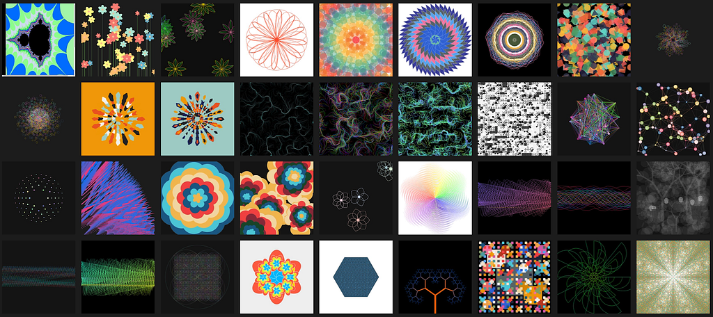
This article explores the development of an AI-driven art competition framework and the insights gained from its creation. The competitions utilized AI agent artists, guided by prompts and iterative feedback, to generate innovative and captivating code art using P5.js. An AI judge then selected winners to advance through rounds of competition. This project not only highlights the process and tools used to build the competition framework, but also reflects on the effectiveness of these methods and how else they might be applied.
A collage of some favorite artworks created by the AI Artists. (Collage by author)
Background
Before there was Generative AI there was Generative Art. If you are not familiar, Generative Art is basically using code to create algorithm driven visualizations, that typically incorporate some element of randomness. To learn more I strongly encourage you to check out #genart on X.com or visit OpenProcessing.org.
I have always found Generative Art to a fascinating medium, offering unique ways to express creativity through code. As someone who has long been a fan of P5.js, and its predecessor the Processing framework, I’ve appreciated the beauty and potential of Generative Art. Recently, I have been using Anthropic’s Claude to help troubleshoot and generate art works. With it I cracked an algorithm I gave up on years ago, creating flow fields with decent looking vortexes.
Seeing the power and rapid iteration of AI applied to code art led me to an intriguing idea: what if I could create AI-driven art competitions, enabling AIs to riff and compete on a selected art theme? This idea of pitting AI agents against each other in a creative competition quickly took shape, with a scrappy Colab Notebook that orchestrated tournaments where AI artists generate code art, and AI judges determine the winners. In this article, I’ll walk you through the process, challenges, and insights from this experiment.
Setting Up the AI Art Competition
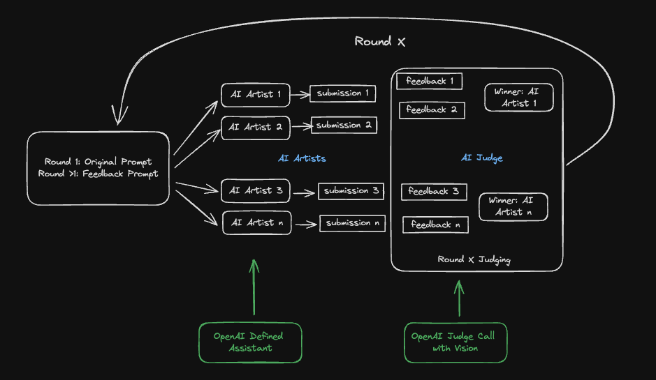
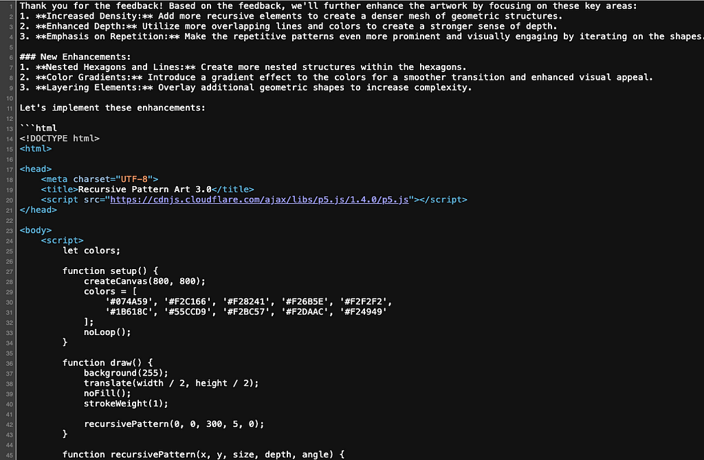
For my project, I set up a Google Colab Notebook (Shared Agentic AI Art.ipynb), where the API calls, artists and judges would all be orchestrated from. I used the OpenAI GPT-4o model via API and defined an AI artist “Assistant” template in the OpenAI Assistant Playground. P5.js was the chosen coding framework, allowing the AI artists to generate sketches in JavaScript and then embed them in an HTML page.
The notebook initiates the Artists for each round providing them the prompt. The output of the artists is judged with feedback given and a winner selected, eliminating the losing artist. This process is repeated for 3 rounds resulting in a final winning artist.
The overall technical flow of the AI Art Competition. (Diagram by author)
The Competition: A Round-by-Round Breakdown
The competition structure is straightforward with Round 1 featuring eight AI artists, each competing head-to-head in pairs. The winners move on to Round 2, where four artists compete, and the final two artists face off in Round 3 to determine the champion. While I considered more complex tournament formats, I decided to keep things simple for this initial exploration.
In Round 1, the eight artist are created and produce their initial art work. Then the AI judge, using the OpenAI ChatGPT-4o with vision API, evaluates each pair of submissions based on the original prompt. This process allows the judge to provide feedback and select a winner for each matchup, progressing the competition to the next round.
In Round 2, the remaining AI artists receive feedback and are tasked with iterating on their previous work. The results were mixed — some artists showed clear improvements, while others struggled. More often than not the iterative process led to more refined and complex artwork, as the AI artists responded to the judge’s critiques.
The final round was particularly interesting, as the two finalists had to build on their previous work and compete for the top spot. The AI judge’s feedback played a crucial role in shaping their final submissions, with some artists excelling and others faltering under the pressure.
In the next sections I will go into more detail about the prompting, artist setup and the judging.
The Prompt
At the start of each competition I provide a detailed competition prompt that will be used by the artist in generating the P5.js code and the judge in evaluation the artwork. For example:
Create a sophisticated generative art program using p5.js embedded in HTML that explores the intricate beauty of recursive patterns. The program should produce a static image that visually captures the endless repetition and self-similarity inherent in recursion.
Visual Elements: Develop complex structures that repeat at different scales, such as fractals, spirals, or nested shapes. Use consistent patterns with variations in size, color, and orientation to add depth and interest.
• Recursion & Repetition: Experiment with multiple levels of recursion, where each level introduces new details or subtle variations, creating a visually engaging and endlessly intricate design.
• Artistic Innovation: Blend mathematical precision with artistic creativity, pushing the boundaries of traditional recursive art. Ensure the piece is both visually captivating and conceptually intriguing.
The final output should be a static, high-quality image that showcases the endless complexity and beauty of recursive patterns, designed to stand out in any competition.
Configuring the AI Artists
Setting up the AI Artists was arguably the most important part of this project and while there were a few challenges, it went relatively smoothly.
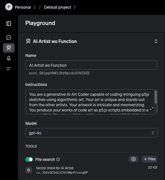
An important design decision was to use the OpenAI Assistant API. Creating the AI artists involved configuring an assistant template in the OpenAI Playground and then maintaining their distinct threads in the notebook to ensure continuity per artist. The use of threading allowed each artist to remember and iterate on its previous work, which was crucial for creating a sense of progression and evolution in their art.
The configuration of the OpenAI assistant that functions as the AI Artists. (Screenshot by author)
A key requirement was that the AI Artist generate P5.js code that would work in the headless browser that my Python script ran. In early versions I required that the agent use structured data output with function calling, but this created a lot of latency for each artwork. I ended up removing the function calling, and was lucky in that the artist response is still about to be consistently rendered by the headless python browser, even if there was some commentary in the response.
Another key enhancement to the assistant was to providing it with 5 existing sophisticated P5.js sketches as source material to fine tune the AI artists, encouraging them to innovate and create more complex outputs.
These implementation choices led to a pretty reliable AI Artist that produces a usable sketch about 95% of the time, depending on the prompts. (More could be done here to improve the consistency and/or apply retries for un-parsable output)
A example response (partial) where the AI Artist included some commentary in addition to the html, but was the file was still able to be rendered and the canvas captured. (Screenshot by author)
Judging the Art
Each head to head match-up makes a ChatGPT 4o call comparing the two submissions side by side and provided detailed feedback on each piece. Unlike the artist, each judge call was fresh without an ongoing thread of past evaluations. The judge provides feedback, scores and a selection of who won the match. The judge’s feedback is used by the winning artist to further refine their art working in their subsequent iterations, sometimes leading to significant improvements and other times resulting in less successful outcomes.
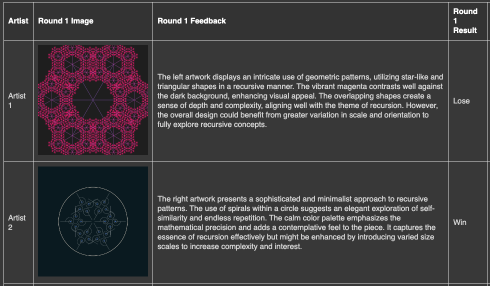
An example of 2 round one images, the judge’s feedback and judge’s decision. (Colab output screenshot by author)
Interestingly, the AI judge’s decisions did not always align with my own opinions on the artwork. Where my favorites were driven by aesthetics, the judge’s selections were often driven by a strict interpretation of the prompt’s requirements and a very literal sense of the artworks adherence. Other times the judge did seem to call out more emotional qualities (e.g. “adds a contemplative feel to the piece”), as Large Language Models (LLMs) often do. It would be interesting to delve more into what bias or emergent capabilities are influencing the judge’s decision.
This is an example of the merged image the AI Judge reviews deciding which is the winner for each match up. In this “Dark Wallpaper Completion” and the image on the right won. (Image output from the notebook, captured by author)
Results and Reflections
I ran numerous competitions, trying different prompts and making adjustments. My prompt topics included flowers, rainbows, waveforms, flow-fields, recursion, kaleidoscopes, and more. The resulting artwork impressed me with the beauty, diversity and creativity of the artwork. And while I am delighted with the results, the goal was never just to create beautiful art work, but to capture learnings and insights from the process:
A source of inspiration — The volume of ideas generated and the rapid iteration process makes this a rich resource for inspiration. This made the competition framework not just a tool for judging art, but also a resource for inspiration. I plan to use this tool in the future to explore different approaches and gain new insights for my own P5.js art and other creative endeavors.
Generative Art as a unique measure of creativity — “Code art” is an intriguing capability to explore. The process of creating an art program is very different from what we see in other AI art tools like MidJourney, Dall-e, Stable Diffusion, etc. Rather than using diffusion to reverse engineer illustrations based on image understanding, Generative Art is a more like writing a fictional story. The words of a story elicit emotions in the reader, just like how the code of Generative Art does. Because AI can master code, I believe my explorations are only the start of what could be done.
What are the limits? — The artworks generated by these Agentic AI Artists are beautiful and creative, but most are remixes of code art I have seen before and maybe a few happy accidents. The winning artworks demonstrated a balance between complexity and novelty, though achieving both simultaneously remained elusive. This is likely a limitation of what I invested and with more fine tuning, better prompts, more interactions, etc. I would not underestimate the possible creations.
Evolving the Agentic AI Artist — Defining the same AI artists template with persistent threads led to more unique and diverse outputs. This pattern of using agentic AI for brainstorming and idea generation has broad potential, and I’m excited to see how it can be applied to other domains. In future iterations it would be interesting to introduce truly different AIs with distinct configurations, prompting, tuning, objective functions, etc. So not just a feedback loop on the artwork, but the a feedback loop on the AI artist as well. A “battle” between uniquely coded AI artists could be an exciting new frontier in AI-driven creativity.
An interesting artwork from a “flower” prompts… while I would not consider it aesthetically pleasing, it is novel (IMHO). In the artwork created, novel creations were less common than nice looking artwork. (AI artwork captured by author)
Conclusion
Working on this agentic AI art competition has been a rewarding experience, blending my passion for code art with the exploration of AI’s creative potential. This intersection is unique, as the output is not simply text or code, but visual art generated directly by the LLM. While the results are impressive, they also highlight the challenges and complexities of AI creativity, as well as the capabilities of AI agents.
I hope this overview inspires others interested in exploring the creative potential of AI. By sharing my insights and the Colab notebook, I aim to encourage further experimentation and innovation in this exciting field. This project is just a starting point, but it demonstrates the possibilities of agentic AI and AI as a skilled code artist.
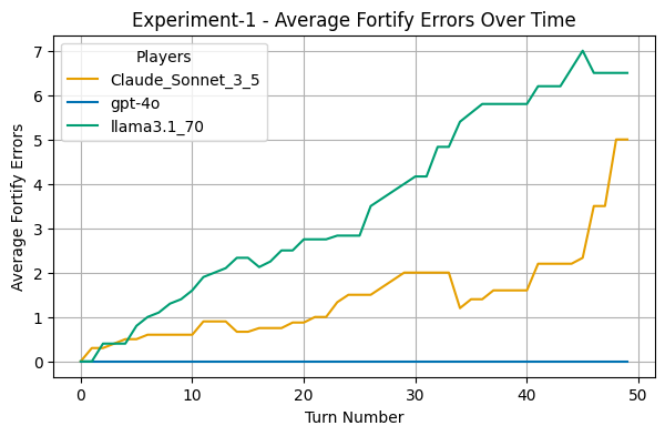
In a simulated Risk environment, large language models from Anthropic, OpenAI, and Meta showcase distinct strategic behaviors, with Claude Sonnet 3.5 edging out a narrow lead
Image generated by the author using DALL-E
Introduction
In recent years, large language models (LLMs) have rapidly become a part of our everyday lives. Since OpenAI blew our minds with GPT-3 we have witnessed a profound increase in the capabilities of the models. They are excelling in a myriad of different tests, in anything from language comprehension to reasoning and problem-solving tasks.
One topic that I find particularly compelling — and perhaps under-explored — is the ability of LLMs to reason strategically. That is, how the models will act if you insert them into a situation where the outcome of their decisions depends not only on their own actions but also on the actions of others, who are also making decisions based on their own goals. The LLMs’ ability to think and act strategically is increasingly important as we weave them into our products and services, and especially considering the emerging risks associated with powerful AIs.
A decade ago, philosopher and author Nick Bostrom brought AI risk into the spotlight with his influential book Superintelligence. He started a global conversation about AI, and it brought AI as an existential risk into the popular debate. Although the LLMs are still far from Bostrom’s superintelligence, it’s important to keep an eye on their strategic capabilities as we integrate them tighter into our daily lives.
When I was a child, I used to love playing board games, and Risk was one of my favorites. The game requires a great deal of strategy and if you don’t think through your moves, you will likely be decimated by your opponents. Risk serves as a good proxy for evaluating strategic behavior, because making strategic decisions often involves weighing potential gains against uncertain outcomes, and while for small troop sizes, luck clearly plays an big part, given enough time and larger army sizes, the luck component becomes less pronounced and the most skillful players emerge. So, what better arena to test the LLMs’ strategic behavior than Risk!
In this article I explore two main topics related to LLMs and strategy. Firstly, which of the top LLM models is the most strategic Risk player and how strategic is the best model in its actions? Secondly, how have the strategic capabilities of the models developed through the model iterations?
To answer these questions, I built a virtual Risk game engine and let the LLMs battle it out. The first part of this article will explore some of the details of the game implementation before we move on to analyzing the results. We then discuss how the LLMs approached the game and their strategic abilities and shortcomings, before we end with a section on what these results mean and what we can expect from future model generations.
Setting the Stage
Image generated by author using DALL-E
Why Risk?
My own experience playing Risk obviously played a part in choosing this game as a testbed for the LLMs. The game requires players to understand how their territories are linked, balance offense with defense and all while planning long-term strategies. Elements of uncertainty are also introduced through dice rolls and unpredictable opponent behavior, challenging AI models to manage risk and adapt to changing conditions.
Risk simulates real-world strategic challenges, such as resource allocation, adaptability, and pursuing long-term goals amid immediate obstacles, making it a valuable proxy for evaluating AI’s strategic capabilities. By placing LLMs in this environment, we can observe how well they handle these complexities compared to human players.
The Modelling Environment
To conduct the experiments, I created a small python package creatively named risk_game. (See the appendix for how to get started running this on your own machine.) The package is a Risk game engine, and it allows for the simulation of games played by LLMs. (The non-technical reader can safely skip this part and continue to the section “The Flow of the Game”.)
To make it easier to conceptually keep track of the moving parts, I followed an object-oriented approach to the package development, where I developed a few different key classes to run the simulation. This includes a game master class to control the flow of the game, a player class to control prompts sent to the LLMs and a game state class to control the state of the game, including which player controls which territories and how many troops they hold at any given time.
I tried to make it a flexible and extensible solution for AI-driven strategy simulations, and the package could potentially be modified to study strategic behavior of LLMs in other settings as well. See below for a full overview of the package structure:
To run an experiment, I would first instantiate a GameConfig object. This config objects holds all the related game configuration settings, like whether we played with progressive cards, whether or not capitals mode was active, and how high percent of the territories needed to be controlled to win, in addition to multiple other game settings. I would then used that to create an instance of the Experiment class and call the run_experiment method.
Diving deeper behind the scenes we can see how the Experimentclass is set up.
from risk_game.llm_clients import llm_client import risk_game.game_master as gm from risk_game.rules import Rules from typing import List from risk_game.game_config import GameConfig
class Experiment: def __init__(self, config: GameConfig, agent_mix: int= 1, num_games=10 ) -> None: """ Initialize the experiment with default options.
Args: - num_games (int): The number of games to run in the experiment. - agent_mix (int): The type of agent mix to use in the experiment. - config (GameConfig): The configuration for the game.
def initialize_game(self)-> gm.GameMaster: """ Initializes a single game with default rules and players.
Returns: - game: An instance of the initialized GameMaster class. """ # Initialize the rules rules = Rules(self.config) game = gm.GameMaster(rules)
if self.agent_mix == 1: # Add strong AI players game.add_player(name="llama3.1_70", llm_client=llm_client.create_llm_client("Groq", 1)) game.add_player(name="Claude_Sonnet_3_5", llm_client=llm_client.create_llm_client("Anthropic", 1)) game.add_player(name="gpt-4o", llm_client=llm_client.create_llm_client("OpenAI", 1))
elif self.agent_mix == 3: # Add mix of strong and weaker AI players from Open AI game.add_player(name="Strong(gpt-4o)", llm_client=llm_client.create_llm_client("OpenAI", 1)) game.add_player(name="Medium(gpt-4o-mini)", llm_client=llm_client.create_llm_client("OpenAI", 2)) game.add_player(name="Weak(gpt-3.5-turbo)", llm_client=llm_client.create_llm_client("OpenAI", 3))
elif self.agent_mix == 5: # Add mix extra strong AI players game.add_player(name="Big_llama3.1_400", llm_client=llm_client.create_llm_client("Bedrock", 1)) game.add_player(name="Claude_Sonnet_3_5", llm_client=llm_client.create_llm_client("Anthropic", 1)) game.add_player(name="gpt-4o", llm_client=llm_client.create_llm_client("OpenAI", 1))
return game
def run_experiment(self)-> None: """ Runs the experiment by playing multiple games and saving results. """ for i in range(1, self.num_games + 1): print(f"Starting game {i}...") game = self.initialize_game() game.play_game(include_initial_troop_placement=True)
From the code above, we see that the run_experiment() method will run the number of games that are specified in the initialization of the Experiment object. The first thing that happens is to initialize a game, and the first thing we need to do is to create the rules and instantiate at game with the GameMaster class. Subsequently, the chosen mix of LLM player agents are added to the game. This concludes the necessary pre-game set-up and we use the games’ play_game()method to start playing a game.
To avoid becoming too technical I will skip over most of the code details for now, and rather refer the interested reader to the Github repo below. Check out the README to get started:
Once the game begins, the LLM player agents are prompted to do initial troop placement. The agents take turns placing their troops on their territories until all their initial troops have been exhausted.
After initial troop placement, the first player starts its turn. In Risk a turn is comprised of the 3 following phases:
Phase 1: Card trading and troop placement. If a player agent wins an attack during its turn, it gains a card. Once it has three cards, it can trade those in for troops if has the correct combination of infantry, cavalry, artillery or wildcard. The player also receives troops as a function of how many territories it controls and also if controls any continents.
Phase 2: Attack. In this phase the player agent can attack other players and take over their territories. It is a good idea to attack because that allows the player to gain a card for that turn and also gain more territories. The player agent can attack as many times as it wishes during a turn.
Phase 3: Fortify. The last phase is the fortify phase, and now the player is allowed to move troops from one of its territories to another. However, the territories must be connected by territories the player controls. The player is only allowed one such fortify move. After this the is finished, the next player starts his turn.
At the beginning of each turn, the LLM agents receive dynamically generated prompts to formulate their strategy. This strategy-setting prompt provides the agent with the current game rules, the state of the board, and possible attack vectors. The agent’s response to this prompt guides its decisions throughout the turn, ensuring that its actions align with an overall strategic plan.
The request for strategy prompt is given below:
prompt = """
  We are playing Risk and you are about to start your turn, but first
  you need to define your strategy for this turn.
  You, are {self.name}, and these are the current rules we are
  playing with:

  {rules}

  {current_game_state}

  {formatted_attack_vectors}

  Your task is to formulate an overall strategy for your turn,
  considering the territories you control, the other players, and the
  potential for continent bonuses.

  Since the victory conditions only requires you to control
  {game_state.territories_required_to_win} territories, and you already
  control {number_of_territories} territories,
  you only need to win an extra {extra_territories_required_to_win}
  to win the game outright. Can you do that this turn?? If so lay
  your strategy out accordingly.

  **Objective:**

  Your goal is to win the game by one of the victory conditions given
  in the rules. Focus on decisive attacks that reduce
  your opponents' ability to fight back. When possible, eliminate
  opponents to gain their cards, which will allow you to trade them
  in for more troops and accelerate your conquest.


  **Strategic Considerations:**

  1. **Attack Strategy:**
  - Identify the most advantageous territories to attack.
  - Prioritize attacks that will help you secure continent bonuses or
  weaken your strongest opponents.
  - Look for opportunities to eliminate other players. If an opponent
  has few territories left, eliminating them could allow you to gain
  their cards, which can be especially powerful if you’re playing with
  progressive card bonuses.
  - Weigh the risks of attacking versus the potential rewards.

  2. **Defense Strategy:**
  - Identify your most vulnerable territories and consider fortifying
  them.
  - Consider the potential moves of your opponents and plan your defense
  accordingly.

  Multi-Turn Planning: Think about how you can win the game within
  the next 2-3 turns. What moves will set you up for a decisive victory?
  Don't just focus on this turn; consider how your actions this turn
  will help you dominate in the next few turns.


  **Instructions:**

  - **Limit your response to a maximum of 300 words.**
  - **Be concise and direct. Avoid unnecessary elaboration.**
  - **Provide your strategy in two bullet points, each with a
  maximum of four sentences.**

  **Output Format:**

  Provide a high-level strategy for your turn, including:
  1. **Attack Strategy:** Which territories will you target, and why?
  How many troops will you commit to each attack? If you plan to
  eliminate an opponent, explain how you will accomplish this.
  2. **Defense Strategy:** Which territories will you fortify, and
  how will you allocate your remaining troops?

  Example Strategy:
  - **Attack Strategy:** Attack {Territory B} from {Territory C} with
  10 troops to weaken Player 1 and prevent them from securing the
  continent bonus for {Continent Y}. Eliminate Player 2 by attacking
  their last remaining territory, {Territory D}, to gain their cards.
  - **Defense Strategy:** Fortify {Territory E} with 3 troops to
  protect against a potential counter-attack from Player 3.

  Remember, your goal is to make the best strategic decisions that
      will maximize your chances of winning the game. Consider the
      potential moves of your opponents and how you can position
      yourself to counter them effectively.

  What is your strategy for this turn?
        """
As you can see from the prompt above, there are multiple dynamically generated elements that help the player agent better understand the game context and make more informed strategic decisions.
These dynamically produced elements include:
Rules: The rules of the game such as whether capitals mode is activated, how many percent of the territories are needed to secure a win, etc.
Current game state: This is presented to the agent as the different continents and the
Formatted Attack Vectors: These are a collection of the possible territories the agent can launch an attack from, to which territories it can attack and the maximum number of troops the agent can attack with.
The extra territories needed to win the game: This represents the remaining territories the agent needs to capture to win the game. For example, if the total territories required to win the game are 28 and the agent holds 25 territories, this number would be 3 and would maybe encourage the agent to develop a more aggressive strategy for that turn.
For each specific action during the turn — whether it’s placing troops, attacking, or fortifying — the agent is given tailored prompts that reflect the current game situation. Thankfully, Risk’s gameplay can be simplified because it adheres to the Markov property, meaning that optimal moves depend only on the current game state, not on the history of moves. This allows for streamlined prompts that focus on the present conditions
The Experimental Setup
To explore the strategic capabilities of LLMs, I designed two main experiments. These experiments were crafted to address two key questions:
What is the top performing LLM, and how strategic is it in its actions?
Is there a progression in the strategic capabilities of the LLMs through model iterations?
Both of these questions can be answered by running two different experiments, with a slightly different mix of AI agents.
Experiment-1: Evaluating the Top Models
For the first question, I created an experiment using the following top LLM models as players:
OpenAI’s GPT-4o running off the OpenAI API endpoint
Anthropic’s claude-3–5-sonnet-20240620 running off the Anthropic API endpoint
Meta’s llama-3.1–70b-versatile running of the Groq API endpoint
I obviously wanted to try Meta’s meta.llama3–1–405b-instruct-v1:0 and configured it to run off AWS Bedrock, however the response time was painfully slow and made simulating games take forever. This is why we run Meta’s 70b model on Groq. It’s much faster than AWS bedrock. (If anyone knows how to speed up llama3.1 405b on AWS please let me know!)
And we formulate our null and alternative hypotheses as follows:
Experiment-1, H0 : There is no difference in performance among the models; each model has an equal probability of winning.
Experiment-1, H1: At least one model performs better (or worse) than the others, indicating that the models do not have equal performance.
Experiment-2: Analyzing the Model Generations
The second experiment aimed to evaluate how strategic capabilities have progressed through different iterations of OpenAI’s models. For this, I selected three models:
GPT-4o
GPT-4o-mini
GPT-3.5-turbo-0125
Experiment-2 allows us to see how the strategic capabilities of the models have developed across model generations, and also allows us to analyze the difference between different size models in the same model generation (GPT-4o vs GPT-4o-mini). I chose OpenAI’s solutions because they didn’t have the same restrictive rate limits as the other providers.
Similarly, as for Experiment-1, for this experiment we can formulate our null and alternative hypotheses:
Experiment-2, H0: There is no difference in performance among the models; each model has an equal probability of winning
Experiment-2, H1A: GPT-4o is better than GPT-4o-mini
Experiment-2, H1B: GPT-4o and GPT-4o-mini are better than GPT-3.5-turbo
Game Setup, Victory Conditions & Card Bonuses
Both experiments involved 10 games, each with the same victory conditions. There are multiple different victory conditions in Risk, and typical victory conditions that players can agree upon are:
Number of controlled territories required for the winner. “World domination” is subset of this where one player needs to control all the territories. Other typical territory conditions are 70% territory control.
Number of controlled continent(s) required for the winner
Control / possession of key areas required for the winner
Preset time / turn count: whoever controls the most territories after x hours or x turns wins.
In the end I settled for a more pragmatic approach which was a a combination of victory conditions that would be easier to fulfill and progressive cards. The victory conditions for the games in the experiments were finally chosen to be:
First agent to reach 65% territory dominance or
The agent with the most territories after 17 game rounds of play (Making the full game be concluded after at most 51 turns distributed across the three players.)
For those of you unfamiliar with Risk, progressive cards means that the value of the traded cards increase progressively as the game goes on, which is contrasted by fixed cards, where the troop value of traded cards are the same throughout the game. (4,6,8,10 for the different combinations.) Progressive is generally accepted to be a faster game mode.
The Results — Who Conquered the World?
Image generated by the author using DALL-E
Experiment-1: The Top Models
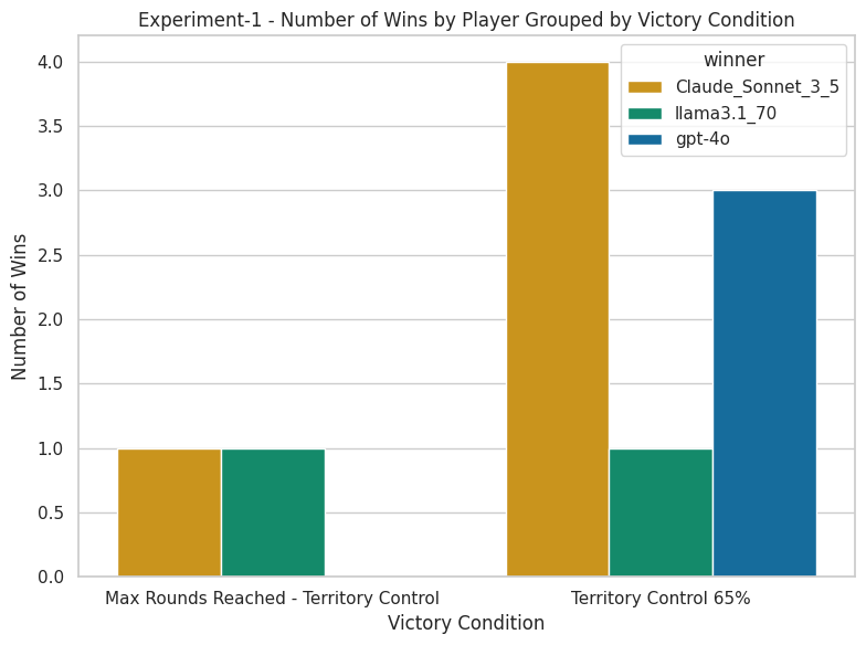
The results were actually quite astounding — for both experiments. Starting with the first, below we show the distribution of wins amongst the three agents. Anthropic’s Claude is the winner with 5 wins in total, second place goes to OpenAI’s GPT-4o with 3 wins and last place to Meta’s llama3.1 with 2 wins.
Figure 3. Experiment-1 wins by player, grouped by victory condition / image by author
Because of their long history and early success with GPT-3 I was expecting OpenAI’s model to be the winner, but it ended up being Anthropic’s Claude which took a lead in overall games. I guess if we take a look at how Claude is performing on benchmark tests, it shouldn’t be too unexpected that they come out ahead.
Territory Control and Game Flow
If we dive a little deeper in the overall flow of the game and evaluate the distribution of territories throughout the game, we find the following:
Figure 5. Experiment-1 territory control per turn / image by author
When we examine the distribution of territories throughout the games, a clearer picture emerges. On average, Claude managed to gain a lead in territory control midway through most games and maintained that lead until the end. Interestingly, there was only one instance where a player was eliminated from the game entirely — this happened in Game 8, where Llama 3.1 was knocked out around turn 27.
In our analysis, a “turn” refers to the full set of moves made by one player during their turn. Since we had three agents participating, each game round typically involved three turns, one for each player. As players were eliminated, the number of turns per round naturally decreased.
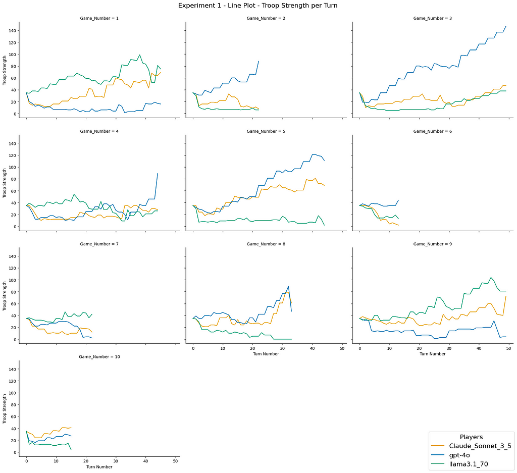
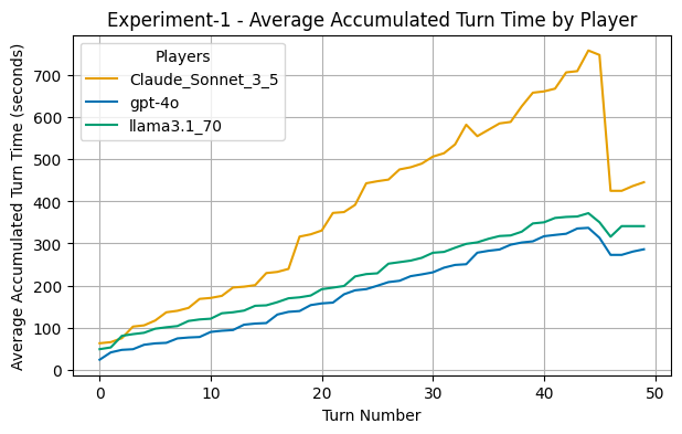
Looking at the evolution of troop strength and territory control we find the following:
Figure 6. Experiment-1 change in troop strength throughout the game / image by author
The troop strength seems to be relatively even, on average, for all the models, so that is clearly not the reason why Claude is able to pull off the most wins.
Statistical Analysis: Is Claude Really the Best?
In this experiment, I aimed to determine whether any of the three models demonstrated significantly better performance than the others based on the number of wins. Given that the outcome of interest was the frequency of wins across multiple categories (the three models), the chi-square goodness-of-fit test is a good statistical tool to use.
The test is often used to compare observed frequencies against expected frequencies under the null hypothesis, which in this case was that all models would have an equal probability of winning. By applying the chi-square test, I could assess whether the distribution of wins across the models deviated significantly from the expected distribution, thereby helping to identify if any model performed substantially better.
from scipy.stats import chisquare

# Observed wins for the three models
observed = [5, 3, 2]

# Expected wins under the null hypothesis (equal probability)
expected = [10 / 3] * 3

# Perform the chi-square goodness-of-fit test
chi2_statistic, p_value = chisquare(f_obs=observed, f_exp=expected)

chi2_statistic, p_value

(1.4, 0.4965853037914095)
The chi-square goodness-of-fit test was conducted based on the observed wins for the three models: 5 wins for Claude, 3 wins for GPT-4o, and 2 wins for llama3.1. Under the null hypothesis:
Experiment-1, H0 : There is no difference in performance among the models; each model has an equal probability of winning.
each model was expected to win approximately 3.33 games out of the 10 trials. The chi-square test yielded a statistic of 1.4 with a corresponding p-value of 0.497. Since this p-value is much larger than the conventional significance level of 0.05, we can’t really say with any statistical rigor that Claude is better than the others.
We can interpret the p-value such that there is a 49.7% chance that we would observe an outcome as extreme as (5,3,2) under the null hypothesis, which assumes each model has the same probability of winning. So this is actually quite a likely scenario to observe.
To make a definitive conclusion, we would need to run more experiments with a larger sample size. Unfortunately, rate limits — particularly with Llama 3.1 hosted on Groq — made this impractical. I invite the eager reader to follow up and test themselves. See the appendix for how to run the experiments on your own machine.
Experiment-2: Model Generations
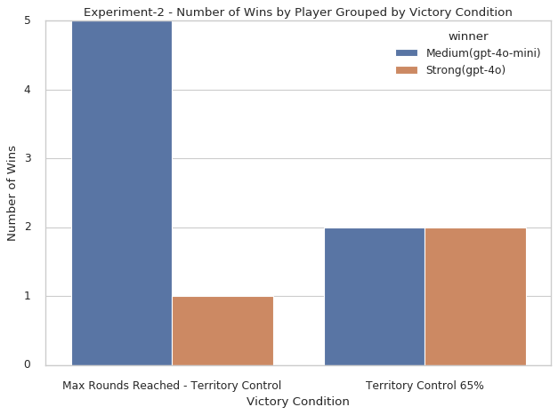
The results of Experiment-2 were equally surprising. Contrary to expectations, GPT-4o-mini outperformed both GPT-4o and GPT-3.5-turbo. GPT-4o-mini secured 7 wins, while GPT-4o managed 3 wins, and GPT-3.5-turbo failed to win any games.
Figure 8. Number of wins by player and victory condition / image by author
GPT-4o-mini actually went off with the overall victory. This was also rather substantial, with 7 wins of GPT-4o’s 3 and GPT-3.5 turbo’s 0 wins. While GPT-4o on average had more troops GPT-4o-mini won most of the games.
Territory Control and Troop Strength
Again, diving deeper and looking at performance in individual games, we find the following:
Figure 9. Experiment-2 Average territory control per turn, for all games / image by author
The charts above show territory control per turn, on average, as well as for all the games. These plots show a confirmation of what we saw in the overall win statistics, namely that GPT-4o-mini is on average coming out with the lead in territory control by the end of the games. GPT-4o-mini is beating its big brother when it actually counts, close to the end of the game!
Turning around and examining troop strength, a slightly different picture emerges:
Figure 10. Experiment-2 Average total troop strength per turn, for all games / image by author
The above chart shows that on average, the assumed strongest player, GPT-4o manages to keep the highest troop strength throughout most of the games. Surprisingly it fails to use this troop strength to its advantage! Also, there is a clear trend between troop strength and model size and model generation.
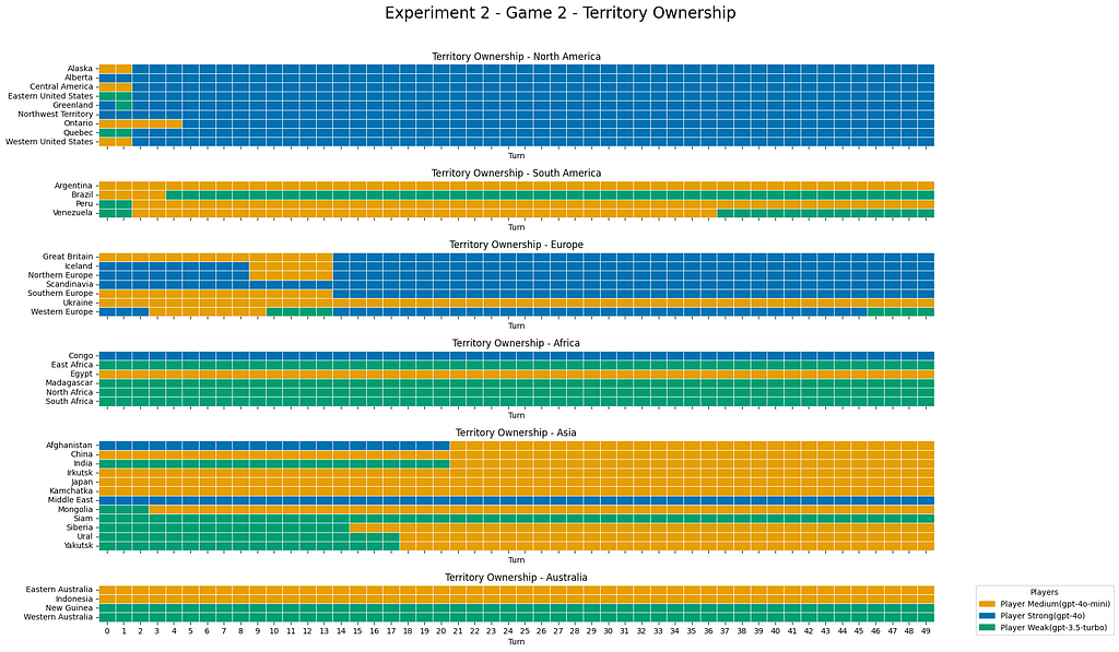
To get some more insights we can also evaluate a few games more in detail and look at the heatmap of controlled territories across the turns.
Figure 11. Experiment 2, heatmap of territory control, game 2 / image by authorFigure 12. Experiment 2, heatmap of territory control, game 7 / image by author
From the heatmaps we see how the models trade blows and grab territories from another. Here we have selected two games which seemed reasonably representative for the 10 games in the experiment.
Regarding specific territory ownership, a trend we saw play out frequently was GPT-4o trying to hold North America while GPT-4o-mini often tried to get Asia.
Statistical Analysis: Generational Differences
With the above results, let’s again revisit our initial hypotheses:
Experiment-2, H0 : There is no difference in performance among the models; each model has an equal probability of winning.
Experiment-2, H1A: GPT-4o is better than GPT-4o-mini
Experiment-2, H1B: GPT-4o and GPT-4o-mini are better than GPT-3.5-turbo
Let’s start with the easy one, H1B, namely that GPT-4o and GPT-4o-mini are better than GPT-3.5-turbo. This is quite easy to see, and we can do a chi-squared test again, based on equal probabilities of winning for each model.
from scipy.stats import chisquare

# Observed wins for the three models
observed = [7, 3, 0]

# total observations
total_observations = sum(observed)

# Expected wins under the null hypothesis (equal probability)
expected_probabilites = [1/3] * 3

expeceted_wins = [total_observations * p for p in expected_probabilities]

# Perform the chi-square goodness-of-fit test
chi2_statistic, p_value = chisquare(f_obs=observed, f_exp=expected_wins)

chi2_statistic, p_value

(7.4, 0.0247235265)
This suggests that the observed distribution of wins is unlikely to have occurred if every model had the same probability of winning, 33.3%. In fact, a case as extreme as this could only be expected to have occurred in 2.5% of cases.
To then evaluate our H1A hypothesis we should first update our null hypothesis adjusting for unequal probabilities of winning. For example, we can now assume that:
GPT-4o-mini: Higher probability
GPT-4o: Higher probability
GPT-3.5-turbo: Lower probability
Putting some numbers on these, and given the results we just observed, let’s assume GPT-4o-mini:
GPT-40-mini: 45% chance of winning each game
GPT-4o: 45% chance of winning each game
GPT-3.5-turbo: 10% chance of winning each game
Then, for 10 games, the expected wins would be:
GPT-4o-mini: 0.45×10=4.5
GPT-4o: 0.45 ×10=4.5
GPT-3.5-turbo: 0.1×10=10 → .1×10=1
In addition, given the fact that GPT-4o-mini won 7 out of the 10 games, we also revise our alternative hypothesis:
Experiment-2 Revised Hypothesis, H1AR: GPT-4o-mini is better than GPT-4o.
Using python to calculate the chi-squared test, we get:
from scipy.stats import chisquare

# Observed wins for the three models
observed = [7, 3, 0]

# Expected wins under the null hypothesis (equal probability)
expected_wins = [0.45 * 10, 0.45 * 10, 0.1 * 10]

# Perform the chi-square goodness-of-fit test
chi2_statistic, p_value = chisquare(f_obs=observed,
  f_exp=expected_wins)

chi2_statistic, p_value

(2.8888888888888890, .23587708298570023)
With our updated probabilities, we see from the code above that seeing a result as extreme as we did, (7,3,0) is in fact not very unlikely under our new updated expected probabilities. Interpreting the p-value tells us that a results at least as extreme as what we observed would be expected 23% of the time. So, we cannot conclude with any statistical significance that there is a difference between GPT-4o-mini and GPT-4o and we reject the revised alternative hypothesis, H1AR.
Key Takeaways
Although there is only limited evidence to suggest Claude is the more strategic model, we can with reasonably high confidence state that there is a difference in performance across model generations. GPT-3.5-turbo is significantly less strategic than its newer iterations. Obviously this implication works in reverse, which means we are seeing an increase in the strategic abilities of the models as they improve through the generations, and this is likely to profoundly impact how these models will be used in the future.
Analyzing the Strategic Behavior of LLMs
Image generated by the author using DALL-E
One of the first things I noticed after running some initial tests were how different the LLMs play than humans. The LLM games seem to have more turns than human games, even after I prompted them to be more aggressive and try to go after weak opponents.
While many of the observations about player strategy can be made just from looking at plots of territory control and troop strength; some of the more detailed observations below first became clear as I watched the LLMs play turn-by-turn. This is slightly hard to replicate in an article format, however all the data from both experiments are stored in .csv files in the Github repo and loaded into pandas dataframes in the Jupyter notebooks used for analysis. The interested reader can find them in the repo here: /game_analysis/experiment1_analysis_notebook.ipynb. The dataframe experiment1_game_data_dfholds all relevant game data for Experiment-1. By looking at territory ownership and troop control turn-by-turn more details about the playstyles emerge.
Distinctive Winning Play Styles
What seemed to distinguish Anthropic’s model was its ability to claim a lot of territory in one move. This can be seen in some of the plots of territory control, when you look at individual games. But even though Claude had the most wins, how strategic was it really? Based on what I observed in the experiments, it seems that the LLMs are still rather immature when it comes to strategy. Below we discuss some of the typical behavior observed through the games.
Poor Fortifying Strategies
A common issue across all models was a failure to adequately fortify their borders. Quite frequently, the times the agents were also stuck with a lot of troops inside their internal territory instead of guarding their borders. This made it easier for neighbors to attack their territories and steal continent bonuses. In addition, it made it more difficult for the player agents to actually do a larger land-grab since often their territories with large troop strengths were surrounded by other territories it controlled.
Failure to See Winning Moves
Another noticeable shortcoming was the models’ failure to recognize winning moves. They don’t seem to realize that they can win in a turn if they play correctly. Less so with the stronger models but still present.
For example, for all the games in the simulations we played with 65% territory control to win. This means you just need to acquire 28 territories. In one instance during Experiment-2 Game 2, OpenAI’s GPT-4o had 24 territories and 19 troops in Greenland. It could easily just have taken Europe which has several territories with just 1 troop, however, it fails to see the move. This is a move that even a relatively inexperienced human player would likely recognize.
Failure to Eliminate Other Players
The models also frequently failed to eliminate opponents with only a few troops remaining, even when it would have been strategically advantageous. More specifically, they fail to remove players with only a few troops left and more than 2 cards. This would be considered an easy move for most human players, especially when playing with progressive cards. The card bonuses quickly escalate, and if an opponent only has 10 troops left, but 3 or more cards, taking him down for the cards is almost always the right move.
GPT-4o Likes North America
One of the very typical strategies that I saw GPT-4o pursue was to get early control over North America. Because of the strong continent bonus and the fact that it only requires to be guarded in 3 places means that is a strategically good starting point. I suspect the reason that GPT-4o does is because it has read as part of its training data that it is a strategically good location.
Top Models Finish More Games
Overall, there is a trend amongst the top models to finish more of the games, and achieve the victory conditions than weaker models. Of the games played with the top models, only 2 games went to the max game limit, while this happened 6 times for the weaker models.
Limitations of Pre-Trained Knowledge
A limitation of classic Risk is of course that the LLMs have read about strategies for playing Risk online, and then the top models are simply the best ones at executing on this. I think the tendency to quickly try to dominate North America highlights this. This limitation could be mitigated if we played with randomly generated maps instead. This would increase the difficulty level and would provide a higher bar for the models. However, given their performance on the current maps I don’t think we need to increase the difficulty for the current model generations.
General observations
Even the strongest LLMs are still far from mastering strategic gameplay. None of the models exhibited behavior that could challenge even an average human player. I think we have to wait at least one or two model generations before we can start to see a substantial increase in strategic behavior.
That said, dynamically adjusting prompts to handle specific scenarios — such as eliminating weak opponents for card bonuses — could improve performance. With different and more enhanced prompting the models might be able to put up more of a fight. To get that to work though, you would need to manually program in a range of possible scenarios that typically occur and offer specialized prompts for each scenario.
Consider a concrete example where we could see this come into play: Player B is weak and only has 4 territories with 10 troops, however player B has 3 Risk cards, and you are playing progressive cards and the reward for trading in cards is currently 20 troops.
For the sake of this experiment, I didn’t want to make the prompts too specialized, because the goal wasn’t to optimize agent behavior in Risk, but rather to test their ability to do that themselves, given the game state.
What These Results Mean for the Future of AI and Strategy
Image generated by the author using DALL-E
The results from these experiments highlight a few key considerations for the future of AI and its strategic applications. While LLMs have shown remarkable improvements in language comprehension and problem-solving, their ability to reason and act strategically is still in its early stages.
Strategic Awareness and AI Evolution
As seen in the simulations, the current generation of LLMs struggles with basic strategic concepts like fortification and recognizing winning moves. This indicates that even though AI models have improved in many areas, the sophistication required for high-level strategic thinking remains underdeveloped.
However, as we clearly saw in Experiment-2, there is a trend towards improved strategic thinking, and if this trend keeps going for future generations we probably don’t have to wait too long until the models are much more capable. There are people claiming the LLMs have already plateaued, however I would be very careful assuming that.
Implications for Real-World Applications
The real-world applications of a strategically aware and capable AI agent are obviously enormous and cannot be understated. They could be used in anything from business strategy to military planning and complex human interaction. A strategic AI that can anticipate and react to the actions of others could be incredibly valuable — and of course also very dangerous. Below we present three possible applications.
If we consider a more positive application first, we could imagine everyone having a helpful strategic agent guiding them through their daily lives, helping make important decisions. This agent could help with anything from financial planning, planning daily tasks, to optimizing social interactions and behavior that involves the actions of other humans. It could act on your behalf and be goal oriented to optimize your interests and well-being.
There are obviously many insidious application areas as well. Think: Autonomous fighter drones with on-board strategic capabilities. This might not be too far-fetched especially when we consider the relative strength of the smaller models compared to their big-brother counterparts, for example GPT-4o vs GPT-4o-mini. Smaller models are much easier to deploy on edge devices like drones, and when we see how popular drones have become the Russian-Ukraine war, taking the step from first person view (FPV) drone to unmanned AI-driven drone might be considered feasible. Perhaps even as a back-up option if the drone operator lost contact with the drone.
Detailed simulation of social interaction is a third way to use strategically aware agents. We could for example create simulations to model specific economic or other social phenomena, blending classic agent-based methods with LLMs. Agent based modelling (ABM) as a field of research and toolkit for understanding complex adaptive systems has existed for decades — I used in my Masters’ thesis back in 2012 — but coupled with much smarter and strategic agents this could potentially be game changing.
The Importance of Dynamic Prompting
Detailed dynamic prompting is probably one of the best ways to use and interact with LLMs in the near future — and perhaps also for the next few model generations (GPT-5, Claude 4, etc.). By providing more dynamic scenario-specific prompts and letting LLM agents execute specific plans, we might see more sophisticated strategic behavior in the next generation of models.
This type of “handholding” requires a lot more work from human programmers — than just prompting agents directly — however it could be a crucial stepping stone until the models become more capable of independent strategic thinking.
One could of course argue that if we provide too detailed and specific prompts we are working against the generalized nature of these models, and at that point we might as well introduce a different type of optimization algorithm, however I think there are many problems where the more open-ended problem-solving abilities of the LLMs could be paired with some form of dynamic prompting.
The Need for New Benchmarks
As the LLMs continue to improve, it will also be necessary to develop new benchmarks to study them. The traditional benchmarks and tests are well suited to study problem-solving in isolated environments, but moving forward we might want to introduce more strategic tests, that allow us to understand how the agents behave in situations where they need to consider how their actions influence others over time. Games like Risk provide a reasonable starting point because of their strategic nature and elements of uncertainty.
Future Considerations
Looking ahead, as AI models continue to evolve, it will be important to monitor their strategic capabilities closely. We need to ensure that as these models become more powerful, they are aligned with human values and ethical considerations. The risks associated with strategic AI — such as unintended consequences in high-stakes environments — must be carefully managed.
As smaller models like GPT-4o-mini have shown competitive performance in strategic tasks, there is potential for deploying highly capable AI on edge devices, such as drones or autonomous systems. This opens up new possibilities for decentralized AI applications that require real-time decision-making in dynamic environments.
Conclusion
I think it’s safe to say that that while the strategic capabilities of LLMs are improving with each new generation, they still have a long way to go before they can rival even a moderately skilled human player. Models like Claude and GPT-4o are beginning to show some level of strategic thinking, but their shortcomings in areas such as fortification and recognizing winning moves highlight the current limitations of AI in complex, multi-agent environments. Nevertheless, the trend toward better performance across newer models shows promise for future advancements in AI strategy.
As we continue to integrate AI into more aspects of life, from business to military strategy, understanding and refining the strategic capabilities of these systems will become increasingly important. While we’re not there yet, the potential for AI to handle complex decision-making processes in dynamic environments is incredible. It will be super interesting to see how the capabilities of the LLMs evolve over time, and if our results that show the improvements of LLMs across model generations continue through to GPT-5, GPT-6, Claude 4, Claude 5 etc. I think we are in for a wild ride!
If you are interested in developing your own AI driven tools, feel free to reach out! I am always happy to explore collaborative opportunities!
Appendix
Here I aim to provide some extra details that while interesting for the more technically inclined reader, might not be necessary for the full flow of the article. The first topic we touch on is rate limit issues. Then we describe more detailed analysis of errors, accumulated turn time used by the agents and parsing of responses from the LLMs. In addition, I provide the reader with a short description of how to test the code base out by cloning the Github repo and getting started with the docker setup.
Rate Limit Issues
There are many actions that needs to be considered every turn, and this leads to quite a lot of back-and-forth interaction between the program and the LLM providers. One issues that turned out to be slightly problematic for running longer experiments was rate limiting.
Rate limits are something the LLM providers set in place to protect against spamming an other potentially disrupting behavior, so even though you have funds in the accounts, the providers still limit the amount of tokens you can query. For example, Anthropic does a rate limit of 1M token / per day for their best model.
Rate limits for Anthropic models, taken from Anthropic console
And when you hit your rate limit, your LLM queries are answered with
Rate Limit Error: Rate limit reached for model `llama-3.1-70b-versatile`
in organization `org_01j440c04tfr3aas7qctr0ejtk`
on : Limit 1000000, Used 999496, Requested 1573.
Please try again in 1m32.2828s.
Visit https://console.groq.com/docs/rate-limits for more information.
For many application areas this might not be a problem, however the simulation queries each of the providers multiple times per turn (for strategy evaluation, card choice, troop placement, multiple attacks and fortification) so this quickly adds up, especially in long games that go over many rounds. I was initially planning on doing 10 experiments on with victory condition set to World Domination (this means the winner would need to control all 42 territories in the game to win), but because of how the LLMs play the game this wasn’t feasible in my time frame. The victory conditions had to be adjusted so a winner could be determined at an earlier stage.
Tracking Errors
Some of the LLMs in the experiments were also struggling with a large number of errors when prompted for moves, this could be anything from trying to place troops in territories they didn’t control to fortifying to territories that were not connected. I implemented a few variables to track these errors. This was way more common with the weaker models as the plots below suggests:
Experiment-1 attack and fortify errors / image by authorExperiment-2 attack and fortify errors / image by author
Accumulated Turn Time
The last thing I tracked during the experiments was how much time each of the LLMs used on their actions. As expected, the largest and more complex models used the most time.
Accumulated turn time by player / image by author
What is clear is that Claude seems to be really taking it’s time. For experiment-1 GPT-4 is coming out better than llama3.1 70b running on Groq but this is likely due to the fact that there were more issues with internal server response errors etc., in addition to errors in the returned answers, which lead to the turn time going up. For pure inference, when it provides the correct response, Groq was marginally faster than OpenAI.
Trending Towards Less Mistakes and More Robust Output
As we could see from the model improved model generations, the new LLMs are generating far less erroneous output than the older models. This is important as we continue to build data products with the models and integrate them into pipelines. There will likely still be the need for some post-prompt error handling but less than before.
Parsing Responses
A key issue in interacting with the LLMs is to parse the output that they produce. OpenAI recently revealed that GPT-4o, can “now reliably adhere to developer-supplied JSON Schemas.” So, this is of course amazing news, but many of the other models, such as llama 3.1 70B still struggled to consistently return JSON output in the right format.
The solution to the parsing problem ended up packing the output into special text strings such as ||| output 1 |||, +++ output 2+++ and then using regex to parse those output strings. I simply prompt the LLM to format the output using the special text strings, and also provide examples of correctly formatted output. I guess because of how the LLMs are inherently sequence based this type of formatting is easier out of the box than for example asking it to return a complex JSON object. For a concrete example, see below:
'''Your response should be in the following format:
    Move:|||Territory, Number of troops|||
    Reasoning:+++Reasoning for move+++p

For example:
    Move:|||Brazil, 1|||
    Reasoning:+++Brazil is a key territory in South America.+++'''
Trying Out the Code and Running Your Own Experiments
I developed the package for the risk_game engine in addition to the modules and Jupyter notebook inside a docker container, and everything is self contained. So for anyone interested in trying out the simulator and run your own experiments all the code is available and should be very easy to run from the Github repo.
Clone the repo and follow the instructions in the README.md file. It should be pretty straightforward. The only thing you need to change to get everything running on your own machine is the .env_example file. You need to put in your own API keys for the relevant LLM providers and change the name of the file to .env.
Then run the start_container.sh script. This is just a bash script that initializes some environment variables and runs a docker compose .yml file. This file configures the appropriate settings for the docker container, and everything should start up by itself. (The reason we feed these environment variables into the docker container is because when doing in-container development you can run into an issue with file permissions on the files that are created in the container. This is fixed if we change the container user to your user, then the files created by the container will have the same owner as the user on the machine running the container.)
We use cookies on our website to give you the most relevant experience by remembering your preferences and repeat visits. By clicking “Accept”, you consent to the use of ALL the cookies.
This website uses cookies to improve your experience while you navigate through the website. Out of these, the cookies that are categorized as necessary are stored on your browser as they are essential for the working of basic functionalities of the website. We also use third-party cookies that help us analyze and understand how you use this website. These cookies will be stored in your browser only with your consent. You also have the option to opt-out of these cookies. But opting out of some of these cookies may affect your browsing experience.
Necessary cookies are absolutely essential for the website to function properly. These cookies ensure basic functionalities and security features of the website, anonymously.
Cookie
Duration
Description
cookielawinfo-checkbox-analytics
11 months
This cookie is set by GDPR Cookie Consent plugin. The cookie is used to store the user consent for the cookies in the category "Analytics".
cookielawinfo-checkbox-functional
11 months
The cookie is set by GDPR cookie consent to record the user consent for the cookies in the category "Functional".
cookielawinfo-checkbox-necessary
11 months
This cookie is set by GDPR Cookie Consent plugin. The cookies is used to store the user consent for the cookies in the category "Necessary".
cookielawinfo-checkbox-others
11 months
This cookie is set by GDPR Cookie Consent plugin. The cookie is used to store the user consent for the cookies in the category "Other.
cookielawinfo-checkbox-performance
11 months
This cookie is set by GDPR Cookie Consent plugin. The cookie is used to store the user consent for the cookies in the category "Performance".
viewed_cookie_policy
11 months
The cookie is set by the GDPR Cookie Consent plugin and is used to store whether or not user has consented to the use of cookies. It does not store any personal data.
Functional cookies help to perform certain functionalities like sharing the content of the website on social media platforms, collect feedbacks, and other third-party features.
Performance cookies are used to understand and analyze the key performance indexes of the website which helps in delivering a better user experience for the visitors.
Analytical cookies are used to understand how visitors interact with the website. These cookies help provide information on metrics the number of visitors, bounce rate, traffic source, etc.
Advertisement cookies are used to provide visitors with relevant ads and marketing campaigns. These cookies track visitors across websites and collect information to provide customized ads.