Tag: artificial intelligence

A simple approach using Monte Carlo simulations

I love games. Chess, Scrabble, you name it. However one that I’m embarrassingly bad at is the very simple game of Connect Four. For some reason, that, and a desire to try my hand at the more practical side of data science, gave me the idea of building a simple AI capable of playing the game of Connect Four at a high skill level.

The obvious problem here is, if I’m terrible at Connect Four, how on Earth can I build an AI capable of playing it? Enter Monte Carlo simulations. Monte Carlo simulations are a powerful tool in data science that use random sampling to estimate complex outcomes. This robust approach has a surprisingly wide array of applications from numerical integration, to financial modelling, and as we’ll explore, playing the game of Connect Four.

In this article I’ll cover a brief introduction to Monte Carlo simulations, then dive into the specifics of making that work for Connect Four, before putting it all together and sharing some code. And if you want, I’ll give you a chance to play the AI yourself and see how you fare.

Let’s go!

Introduction to Monte-Carlo Methods:

That idea of Monte-Carlo sampling is pretty simple — if you have a problem that you cannot solve analytically why not run random experiments and try to estimate a numerical answer? If that does not make sense just yet don’t worry, we’ll look at an example in just a moment. But first, let’s get our history straight.

The backstory of Monte Carlo methods is quite interesting. The primary developer of the method was Stanislaw Ulam, a physicist so prominent he worked on the Manhattan project developing the atomic bomb. Important to our story though was Stanislaw’s uncle, who had an unfortunate gambling habit that led to Stanislaw naming the new calculation method after the famous Monte Carlo casino in Monaco.

Now, back to that example I promised you on just what it means to generate random samples.

A worked example

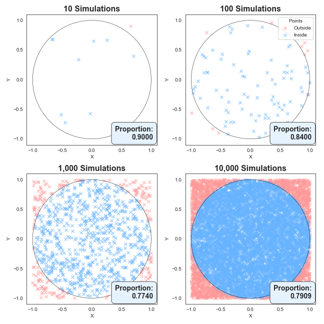
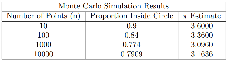
Suppose we want to find the area inside a circle of radius 1. The actual area of such a circle is of course our friend πr² and since r is 1, the area is simply π. But what if we don’t know π – How can we arrive at this answer by generating random experiments as the Monte Carlo method prescribes?

First, simulate random points in the region -1 < x < 1, and -1 < y < 1. Then for each point note whether or not it falls inside or outside the circle. Below I’ve created such simulations for 10, 100, 1000 and 10,000 random coordinates.

What you can see is with only 10 points, the area of the circle (or the proportion that it takes up) is very rough, but as we add more and more points, the proportion of points lying in the circle becomes more consistent.

Now you’re probably asking, well, these charts are pretty and all, but what’s the real takeaway? A very fair question.

Notice we end up with an estimate for the proportion of simulations that results in a point within the circle? Well, we know the area of the square is going to be 2 x 2 = 4, we can then estimate π by multiplying this proportion by 4, because the area is the circle is simply π.

The table below summarises the results. Notice how the π estimate gets closer and closer to the true value as the number of simulations increases.

We can do even better with more simulations of course. The following code snippet that runs one hundred million samples generally gives a number correct to three decimal places:

import numpy as np

n = 100_000_000
points = np.random.rand(n, 2)
inside_circle = np.sum(points[:,0]**2 + points[:,1]**2 <= 1)
pi_estimate = (inside_circle / n) * 4

print(pi_estimate) # prints 3.141x

The key takeaway here is that by generating random simulations (our coordinate pairs), we can achieve a surprisingly precise estimate for a known quantity! Our first example of the Monte Carlo method in action.

Translating the Approach to Games

This is great and all, but we don’t want to calculate π, we want to make an AI capable of playing Connect Four! Fortunately, the logic we just used to calculate π can also be applied to the game of Connect Four.

In the above example we did two things, firstly we generated random samples (coordinate pairs), and then secondly we approximated a quantity (π).

Well here we will do the same. First, we generate random samples as before, but this time those random samples will be choosing random moves, which will simulate entire games of Connect Four.

Then, secondly, we will again approximate a quantity, but the quantity we are chasing is the probability of winning with each move.

A brief refresher of the rules

Before we jump into creating simulations, let’s quickly review the rules of Connect Four. Players take turns dropping their coloured tiles into any unfilled columns on a 7 x 6 game board. The game ends when a player lines up four tiles in any direction, or when the board is full and a draw is reached.

The Monte Carlo method for Connect Four

Okay, now that we are on top of the theory, it’s time to put it into practice and teach an AI to play Connect Four. In order to find the right move in the game of Connect Four we:

1. Randomly sample each of the possible legal moves. (What column to drop a tile into).
2. then simulate the entire game from this point assuming both players make their moves completely at random.
3. Track the outcome of each of the random games to calculate win probabilities for each move.
4. Finally, select the move with the highest win probability.

That sounds quite simple, and in reality it is!

To see this method in action, here is a python implementation of this logic that I have written to play the game of Connect Four. There’s a bit going on, but don’t stress if it doesn’t all make sense — the actual implementation details are less important than the concept!

That said, for those interest the approach makes use of object oriented programming, with a Player class capable of making moves on a Board class.

Here’s how it works in practice: we start with a list of possible valid moves, and we draw from them at random. For each move, we call the `_simulate_move` function, which will simulate an entire game from that point onward and return the winning symbol. If that symbol matches that of the AI player, we increment the wins. After running numerous simulations, we calculate the win rates for each move, and finally return the move corresponding to the highest win rate.

def _get_best_move(self, board: Board, num_sims: int):
    
    # Get a list of all viable moves
    win_counts = {column: 0 for column in range(board.width) if board.is_valid_move(column)}
    total_counts = {column: 0 for column in range(board.width) if board.is_valid_move(column)}
    
    valid_moves = list(win_counts.keys())
    for _ in range(num_sims):
        column = random.choice(valid_moves) # Pick a move a random
        result = self._simulate_move(board, column) # Simulate the game after making the random move
        total_counts[column] += 1
        if result == self.symbol: # Check whether the AI player won
            win_counts[column] += 1
    
    win_rates = {column: win_counts[column] / total_counts[column] if total_counts[column] > 0 else 0 for column in valid_moves}
    best_move = max(win_rates, key=win_rates.get) # Find the move with the best win rate
    return best_move

In summary, by simulating random moves and tracking the game from that point, this Monte Carlo approach helps the AI start to make much smarter moves than if it were just guessing.

Some Practical Examples:

Okay enough code! Let’s put the AI to the test and see how it will perform in a couple of positions. Below we will go through two different positions, and show the outcome of the above block of code. The first situation is quite simple, and the second a bit more nuanced.

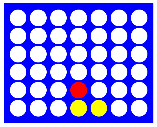
It’s red turn, and the obvious best move is to play a move in the 5th column. If we simulate 1000 random games from this position using the method above, the AI player creates the following win rates. Placing a tile in column 5 results in a win every time (as it should!), and is chosen.

Fantastic! Our AI can identify a winning move when one is available. A simple scenario yes, but to be honest I’ve missed plenty of wins in the game before…

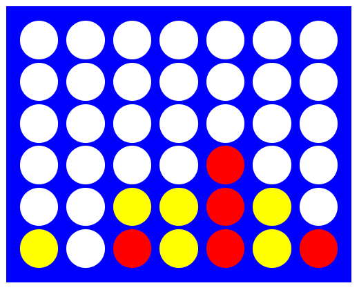
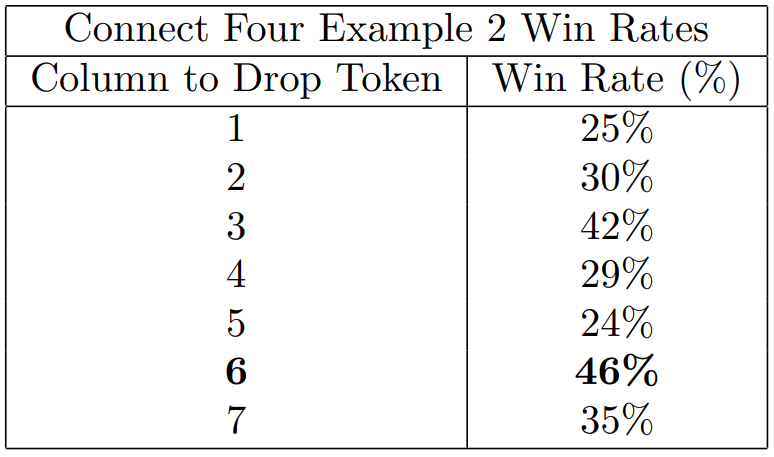
Now, let’s look at another position. This one is a little more tricky. Have you got an idea of what Red should play to prevent Yellow gaining a winning advantage?

The key here is to prevent yellow from creating an open-sided 3 in a row set up, which would lead to a win. Red needs to block this by playing in either the 3rd or 6th column! Simulating 1000 games from this position we get the below win-rates. Note the AI correctly identifies the two blocking moves (column 3 and 6) as having the highest win rates. Further it realised column 6 has the highest chance of winning and selects that.

How does it fair in practice?

See for yourself! You can challenge the AI here: https://fourinarowgame.online/ . The difficulty is based on adjusting the number of simulations. Easy simulates 50 games, moderate simulates 500 games, and hard simulates 1500 games. Personally I can beat the easy mode pretty consistently, but that’s about it!

Conclusion

Okay, let’s bring it all together. In writing this article I really wanted to do two things. First, I wanted to demonstrate the power of the Monte Carlo method for a straight forward calculation like estimating π by simulating random coordinates.

Next, and more interestingly, I wanted to show the strength of the same approach to board games. What’s fascinating is that despite knowing nothing of Connect Four strategy, it’s entirely possible to just simulate random games, and end up with an AI opponent capable of playing at quite a high level!

As always, thanks for reading and see you next time.

---

Beating Connect Four with AI was originally published in Towards Data Science on Medium, where people are continuing the conversation by highlighting and responding to this story.

In this post, we demonstrate how to create an Amazon Q Business application and index website contents using the Amazon Q Web Crawler connector for Amazon Q Business. We use two data sources (websites) here. The first data source is an employee onboarding guide from a fictitious company, which requires basic authentication. We demonstrate how to set up authentication for the Web Crawler. The second data source is the official documentation for Amazon Q Business. For this data source, we demonstrate how to apply advanced settings to instruct the Web Crawler to crawl only pages and links related to Amazon Q Business.

Today, we are happy to announce the general availability of cross-region inference, a powerful feature allowing automatic cross-region inference routing for requests coming to Amazon Bedrock. This offers developers using on-demand inference mode, a seamless solution for managing optimal availability, performance, and resiliency while managing incoming traffic spikes of applications powered by Amazon Bedrock. By opting in, developers no longer have to spend time and effort predicting demand fluctuations.

In this post, we will harness the power of generative artificial intelligence (AI) and Amazon Bedrock to help organizations simplify and effectively manage remediations of AWS Security Hub control findings.

A quick-start tutorial

The landscape of artificial intelligence (AI), particularly in Generative AI, has seen significant advancements recently. Large Language Models (LLMs) have been truly transformative in this regard. One popular approach to building an LLM application is Retrieval Augmented Generation (RAG), which combines the ability to leverage an organization’s data with the generative capabilities of these LLMs. Agents are a popular and useful way to introduce autonomous behaviour into LLM applications.

What is Agentic RAG?

Agentic RAG represents an advanced evolution in AI systems, where autonomous agents utilize RAG techniques to enhance their decision-making and response abilities. Unlike traditional RAG models, which often rely on user input to trigger actions, agentic RAG systems adopt a proactive approach. These agents autonomously seek out relevant information, analyse it and use it to generate responses or take specific actions. An agent is equipped with a set of tools and can judiciously select and use the appropriate tools for the given problem.

This proactive behaviour is particularly valuable in many use cases such as customer service, research assistance, and complex problem-solving scenarios. By integrating the generative capability of LLMs with advanced retrieval systems agentic RAG offers a much more effective AI solution.

Key Features of RAG Using Agents

1.Task Decomposition:

Agents can break down complex tasks into manageable subtasks, handling retrieval and generation step-by-step. This approach enhances the coherence and relevance of the final output.

2. Contextual Awareness:

RAG agents maintain contextual awareness throughout interactions, ensuring that retrieved information aligns with the ongoing conversation or task. This leads to more coherent and contextually appropriate responses.

3. Flexible Retrieval Strategies:

Agents can adapt their retrieval strategies based on the context, such as switching between dense and sparse retrieval or employing hybrid approaches. This optimization balances relevance and speed.

4. Feedback Loops:

Agents often incorporate mechanisms to use user feedback for refining future retrievals and generations, which is crucial for applications that require continuous learning and adaptation.

5. Multi-Modal Capabilities:

Advanced RAG agents are starting to support multi-modal capabilities, handling and generating content across various media types (text, images, videos). This versatility is useful for diverse use cases.

6. Scalability:

The agent architecture enables RAG systems to scale efficiently, managing large-scale retrievals while maintaining content quality, making them suitable for enterprise-level applications.

7.Explainability:

Some RAG agents are designed to provide explanations for their decisions, particularly in high-stakes applications, enhancing trust and transparency in the system’s outputs.

This blog post is a getting-started tutorial which guides the user through building an agentic RAG system using Langchain with IBM Watsonx.ai (both for embedding and generative capabilities) and Milvus vector database service provided through IBM Watsonx.data (for storing the vectorized knowledge chunks). For this tutorial, we have created a ReAct agent.

Step 1: Package installation

Let us first install the necessary Python packages. These include Langchain, IBM Watson integrations, milvus integration packages, and BeautifulSoup4 for web scraping.

%pip install langchain
%pip install langchain_ibm
%pip install BeautifulSoup4
%pip install langchain_community
%pip install langgraph
%pip install pymilvus
%pip install langchain_milvus

Step 2: Imports

Next we import the required libraries to set up the environment and configure our LLM.

import bs4
from Langchain.tools.retriever import create_retriever_tool
from Langchain_community.document_loaders import WebBaseLoader
from Langchain_core.chat_history import BaseChatMessageHistory
from Langchain_core.prompts import ChatPromptTemplate
from Langchain_text_splitters import CharacterTextSplitter
from pymilvus import MilvusClient, DataType
import os, re

Here, we are importing modules for web scraping, chat history, text splitting, and vector storage (milvus)

Step 3: Configuring environment variables

We need to set up environment variables for IBM Watsonx, which will be used to access the LLM which is provided by Watsonx.ai

os.environ["WATSONX_APIKEY"] = "<Your_API_Key>"
os.environ["PROJECT_ID"] = "<Your_Project_ID>"
os.environ["GRPC_DNS_RESOLVER"] = "<Your_DNS_Resolver>"

Please make sure to replace the placeholder values with your actual credentials.

Step 4: Initializing Watsonx LLM

With the environment set up, we initialize the IBM Watsonx LLM with specific parameters to control the generation process. We are using the ChatWatsonx class here with mistralai/mixtral-8x7b-instruct-v01 model from watsonx.ai.

from Langchain_ibm import ChatWatsonx

llm = ChatWatsonx(
    model_id="mistralai/mixtral-8x7b-instruct-v01",
    url="https://us-south.ml.cloud.ibm.com",
    project_id=os.getenv("PROJECT_ID"),
    params={
            "decoding_method": "sample",
            "max_new_tokens": 5879,
            "min_new_tokens": 2,
            "temperature": 0,
            "top_k": 50,
            "top_p": 1,
        }
)

This configuration sets up the LLM for text generation. We can tweak the inference parameters here for generating desired responses. More information about model inference parameters and their permissible values here

Step 5: Loading and splitting documents

We load the documents from a web page and split them into chunks to facilitate efficient retrieval. The chunks generated are stored in the milvus instance that we have provisioned.

loader = WebBaseLoader(
    web_paths=("https://lilianweng.github.io/posts/2023-06-23-agent/",),
    bs_kwargs=dict(
        parse_only=bs4.SoupStrainer(
            class_=("post-content", "post-title", "post-header")
        )
    ),
)
docs = loader.load()
text_splitter = CharacterTextSplitter(chunk_size=1500, chunk_overlap=200)
splits = text_splitter.split_documents(docs)

This code scrapes content from a specified web page, then splits the content into smaller segments, which will later be indexed for retrieval.

Disclaimer: We have confirmed that this site allows scraping, but it’s important to always double-check the site’s permissions before scraping. Websites can update their policies, so ensure your actions comply with their terms of use and relevant laws.

Step 6: Setting up the retriever

We establish a connection to Milvus to store the document embeddings and enable fast retrieval.

from AdpativeClient import InMemoryMilvusStrategy, RemoteMilvusStrategy, BasicRAGHandler

def adapt(number_of_files=0, total_file_size=0, data_size_in_kbs=0.0):
    strategy = InMemoryMilvusStrategy()
    if(number_of_files > 10 or total_file_size > 10 or data_size_in_kbs > 0.25):
        strategy = RemoteMilvusStrategy()
    client = strategy.connect()
    return client

client = adapt(total_size_kb)
handler = BasicRAGHandler(client)
retriever = handler.create_index(splits)

This function decides whether to use an in-memory or remote Milvus instance based on the size of the data, ensuring scalability and efficiency.

BasicRAGHandler class covers the following functionalities at a high level:

· Initializes the handler with a Milvus client, allowing interaction with the Milvus vector database provisioned through IBM Watsonx.data

· Generates document embeddings, defines a schema, and creates an index in Milvus for efficient retrieval.

· Inserts document, their embeddings and metadata into a collection in Milvus.

Step 7: Defining the tools

With the retrieval system set up, we now define retriever as a tool . This tool will be used by the LLM to perform context-based information retrieval

tool = create_retriever_tool(
    retriever,
    "blog_post_retriever",
    "Searches and returns excerpts from the Autonomous Agents blog post.",
)
tools = [tool]

Step 8: Generating responses

Finally, we can now generate responses to user queries, leveraging the retrieved content.

from langgraph.prebuilt import create_react_agent
from Langchain_core.messages import HumanMessage

agent_executor = create_react_agent(llm, tools)

response = agent_executor.invoke({"messages": [HumanMessage(content="What is ReAct?")]})
raw_content = response["messages"][1].content

In this tutorial (link to code), we have demonstrated how to build a sample Agentic RAG system using Langchain and IBM Watsonx. Agentic RAG systems mark a significant advancement in AI, combining the generative power of LLMs with the precision of sophisticated retrieval techniques. Their ability to autonomously provide contextually relevant and accurate information makes them increasingly valuable across various domains.

As the demand for more intelligent and interactive AI solutions continues to rise, mastering the integration of LLMs with retrieval tools will be essential. This approach not only enhances the accuracy of AI responses but also creates a more dynamic and user-centric interaction, paving the way for the next generation of AI-powered applications.

NOTE: This content is not affiliated with or endorsed by IBM and is in no way an official IBM documentation. It is a personal project pursued out of personal interest, and the information is shared to benefit the community.

---

Building an Agentic Retrieval-Augmented Generation (RAG) System with IBM Watsonx and Langchain was originally published in Towards Data Science on Medium, where people are continuing the conversation by highlighting and responding to this story.