In this post, we delve into the process of building and deploying a sample application capable of generating multilingual descriptions for multiple images with a Streamlit UI, AWS Lambda powered with the Amazon Bedrock SDK, and AWS AppSync driven by the open source Generative AI CDK Constructs.
Patterns in performance and reward in the heptathlon and decathlon
Image by author with DALL-E 3
While watching the 2024 Olympic Heptathlon competition, I was reminded that the points scores by event in the heptathlon always show a pattern: the first event, the 100 metres hurdles, usually sees large points numbers across the board, while the shot put, the third event, tends to return a couple of hundred fewer points per athlete.
This prompted me to look at two questions: i) why do the points come out as they do, and ii) does this mean that some events are more important than others, to the end of winning the heptathlon competition? The same questions apply to the decathlon too, of course, and this is also examined here.
Data
I collected the results for the World Championship heptathlon and decathlon competitions from 2007 to 2023 from Wikipedia . These are the elite levels of performance for the two multi-event competitions, so the insights gained from this analysis apply to only this high level and not necessarily to heptathlon or decathlon competitions in general. Details on the scoring systems were found on SportsCalculators, and are originally published by World Athletics.
In the analysis that follows I will use the word ‘score’ to refer to the physical performance mark recorded by the athlete in each event (height, length/distance, or time), and ‘points’ to refer to the number of heptathlon or decathlon points that are received for that score.
Results: Heptathlon
Points spreads
Table 1: Points received by event in World Championship heptathlons. Image by author.
The average (median) number of points received for the heptathlon events in Table 1 shows clearly the pattern we’re talking about: the sprint events (200m and, in particular, 100m hurdles) provide around 200 points more, on average, than do the throwing events (javelin and shot put). This seems surprising, but is not necessarily of any importance, since all athletes are competing in all events, so it is only the points scored relative to one another that matter. The third column in the table above shows the interquartile range of points; that is, the difference between the 25th and 75th percentiles, or, the zone in which the ‘middle half’ of athletes lie. Here we see that the running events show the lowest spreads in points, while the high jump and javelin have the largest ranges. This suggests that the difference between performing quite poorly and quite well (relative to World-Championship-level competitors) is more important, in points terms, in some events that it is in others.
Scoring system
The reason for this effect is the scoring system. The systems for both heptathlon and decathlon have been in their current form since 1984, and use for each event an equation of the form
points = a * (difference between score and reference score b) ^ c
where ‘^’ means ‘to the power of’. Each event therefore requires three coefficients, a, b, and c, to be defined. The values of the coefficients are not comparable individually between events, but the combination of the three creates a points curve for each event, as shown in Figure 1, below. The World Athletics document on the scoring systems explains that one factor in the selection of the coefficients is the world record in each event: it is desired that a world-record performance in any event should yield the same number of points. They note that, in practice, this means that ‘the best scores set in each individual event will vary widely’, but that it is more important that ‘the differences in the scores between different athletes in one event are roughly proportional to the differences in their performances’.
Figure 1: Distribution of scores (black lines, and 10–90th percentile in green), points received (blue lines, y-axis), and world records (red dashed lines), by heptathlon event. Image by author.
The blue lines in Figure 1 show the relationship between score and points in each event. The lines are almost straight, particularly within the green shaded score regions, which is where 80% of scores are contained, meaning that the scoring system can, practically, be regarded as a linear system. (There is a slight upward bend to some of the curves, particularly at the high-score end of the long jump and 800m, which means that exceptional performance is rewarded slightly more than would occur in a truly linear system, but these differences are small and are not the key point of this analysis.)
What is more interesting is the range of points that are realistically available from each event. This is indicated by the vertical arrows, which show the points increase obtained by moving from a score at the 10th percentile (left edge of the green area) to a score at the 90th percentile (right edge of the green area). 8 out of 10 performances occur in these ranges, and anything lower or higher is somewhat exceptional for that event. The size of this points range (the height of the arrow) is clearly larger in some events, most noticeably the javelin, than in others, most noticeably the 100m hurdles. This is almost the same information as seen in the interquartile range numbers earlier.
The position of the world records in each event (dashed red lines) show why the average number of points is lower in the throwing events: the average heptathlete can only throw about 60% as far as the world record (best specialist, single-event athlete) for shot put or javelin, but the same heptathlete can attain a speed of between 85% and 90% of the world record (converted from time) in the 100m hurdles and the 200m.
There could be several reasons for this, but one important follow-on point that it seems fair to assume is that an event in which performances are far from the world record has more potential for improvements than an event in which performances are already close to their ultimate limit. To put this another way, it seems that most heptathletes are able to run fairly well compared to the specialists in those events (including the 800m), but in the javelin, their performances generally show relatively large deficiencies compared to what is possible in the event. Importantly though, as the wider score spread for javelin shows, some heptathletes can throw the javelin fairly well.
To make this more clear, next, I use the distributions of scores in each event to measure the points gain that would result from an athlete improving her performance in the event from the 50th percentile (better than half of her competitors) to the 60th percentile (better than 6 in 10 competitors). The intention with this metric is that this improvement might be equally difficult, or equally achievable, in each event, as it is measured by what other heptathletes have achieved. When finding the percentile levels, to avoid problems with the discrete nature of scores in the high jump (only jumps every 3 cm are possible), the raw scores from each event are modelled as distributions (normal in most cases, and log-normal in the cases of high jump, 100m hurdles, and 800m), and the percentiles computed from these.
Figure 2: Points difference between scores at the 50th and 60th percentiles by heptathlon event. Running, jumping, and throwing events are separated by colour. Image by author.
The results (Figure 2) confirm that improving by the same amount relative to one’s peers earns more points in the field events than in the running events. A 10% improvement relative to the competition in the javelin would be the most beneficial performance gain to make, earning the heptathlete 28 points. Later we will discuss whether or not it is truly as easy to make a 10% throwing improvement as it is to improve scores by 10% in the track events.
Results: Decathlon
Table 2: Points received by event in World Championship decathlons. Image by author.
The picture in the decathlon is broadly similar to that described for the heptathlon. In Table 2, we find that, again, the javelin shows the biggest interquartile range for points scored, followed by the 1500m (which sits much higher up the list than the women’s most similar event, the 800m) and the pole vault. Conversely, the sprint events (100m, 110m hurdles, and 400m) show smaller points spreads. The difference in spreads between the top and bottom events is not quite as severe as it is in the heptathlon.
Figure 3: Distribution of scores (black lines, and 10–90th percentile in green), points received (blue lines, y-axis), and world records (red dashed lines), by decathlon event. Image by author.
The score distributions and points curves (Figure 3) show, through the length of the arrows, the events in which the typical range of scores (the width of the green areas) yields the most points difference: the javelin, pole vault, and some way behind, the discus and 1500m. Again, the sprint hurdles shows a small points spread: the worst hurdlers are not penalised much in comparison to the best hurdlers.
The 1500m sits lowest in points terms of any event, with a 10th percentile performance worth only around 600 points. This is a result of the steepness of the blue line, which dictates how much the decathlete is penalised for each additional second that they are away from the world record. The blue line does not have to look like this, but it does as a result of the choice of the coefficients a, b, and c. On the plus side, the steepness of the line creates a relatively large points difference between different scores in the 1500m, as seen below.
Figure 4: Points difference between scores at the 50th and 60th percentiles by decathlon event. Running, jumping, and throwing events are separated by colour. Image by author.
Using the same technique as before of modelling event scores as distributions (log-normal for 1500m, 110m hurdles, and javelin, and normal for the rest) and computing percentiles, Figure 4 shows the same pattern as the heptathlon events: the same percentage improvement in score yields the most points in javelin, and the fewest points in the sprint events.
Event correlation
The above results suggest that a few of the most technical events should be the ones that athletes focus on to gain points most easily. However, training in one event will naturally lead to improvements in some other events as well (and possibly degrade performance in others), so it is not so simple as to be able to consider each event in isolation. The value of effort spent on one event will depend on both the points gain that is possible in that eventandthe complementary benefits obtained in other, similar events.
Figure 5: Rank correlation between scores in heptathlon events, and between event scores and the inverse of finishing position in the competition. Image by author.
The correlation plot of Figure 5 shows how scores in each of the heptathlon events are correlated with one another. The highest correlations are between the 200m, 100m hurdles, and long jump. This is not surprising, as a good sprinter will likely perform well in all of these events. There are also correlations, though smaller, between scores in long jump and high jump, and in shot put and javelin.
It is notable that the javelin shows the least correlation with the other events overall. This is consistent with it being an event requiring its own specific technique, and a heptathlete does not naturally become much better at the javelin by improving in any other events, except for (somewhat) the shot put. Javelin even shows a small negative correlation with both the 200m and 800m: the better javelin throwers in heptathlon tend to be the worse runners.
Figure 6: Rank correlation between scores in decathlon events, and between event scores and the inverse of finishing position in the competition. Image by author.
In decathlon (Figure 6), the sprint events are correlated with one another, as are shot put and discus, whereas pole vault, javelin, and 1500m show quite weak correlations with almost all of the other events.
This changes the message from the previous section. While improving relative to the rest of the field in javelin, pole vault, or middle distance running should provide the biggest points gain per unit of improvement, the benefit of this is undercut by a possible decrease in performance in other events. On the other hand, improving skill in one of the sprint-based events tends to create gains in similar events at the same time, perhaps making this a more efficient approach to the competitions overall.
Finally, the right-most column in each of the correlation grids (Figures 5 and 6) seems to confirm this. This column shows the correlation between scores in each event and final position in the heptathlon or decathlon competition (multiplied by -1 so that a high finish becomes the largest number). The biggest correlation with position — that is, the event in which the athlete’s score most dictates where they finish in the overall competition — is found in the long jump in both heptathlon and decathlon, followed by hurdles and high jump in heptathlon, and by hurdles and 400m in decathlon. The importance of long jump is likely due to its ‘centrality’ in the competitions: its relatively high correlations with several other events. Conversely, performance in the 1500m is the least correlated with finish position in decathlon. This is probably because the best 1500m runners tend not to hold advantages in other events too, so often end up lower in the overall standings. The decathlon is more often won by a strong sprinter, because this athlete is rewarded several times over for this skill, with points in the 100m, hurdles, 400m, and long jump.
Conclusion
Insights on how best to approach the heptathlon and decathlon turned out different from how I expected at the start of the analysis. Although it seems that effort to improve one’s score in the javelin is the most efficient way to increase total points, the athletes that perform best overall do not tend to do particularly well in javelin. This is likely because the skills required for javelin, and to a lesser extent, pole vault, discus, and high jump, do not transfer well to other events, so the benefit of the effort is limited to a points return in that event only.
It may be speculated that these are the most technically demanding events, in which it is perhaps possible, though difficult, for the athlete to ‘unlock’ big gains in performance through small adjustments in technique, whereas some of the other events are more controlled by strength or fitness, in which only incremental gains are feasible. Probably the difficulty in making those technical improvements, combined with the shared benefits of general fitness improvements, tips the balance in favour of improving scores in the sprint-related events.
This balance is nevertheless controlled by the scoring system. Each of the blue lines in Figures 1 and 3 is anchored at one point by the world record, but the gradient of the line appears to be a choice that could have been made differently. The bigger the gradient, the more emphasis is put on the difference in score between the best and worst athletes in that event. In fact, the large gradients for the javelin and other events may be necessary to balance these more isolated events against the shared benefits of improvements in the sprint events. If the points bars of Figures 2 and 4 were equal across all events, there would be less incentive to focus effort on the technical events in preference to the more intercorrelated sprint events.
There is no likelihood of the multi-event scoring systems changing in the near future. I would suggest that the right-most columns of Figures 5 and 6 show that the systems currently work well, as there are no events that are completely uncorrelated with finish position (which would mean that performance in those events didn’t matter to the overall result). If there were to be changes to the system, it might be a good idea to target more even correlations in this column, which would mean increasing the points gradient in the 800m and 1500m, in particular, to increase the benefit of performing well in these events, at the expense of the long jump and hurdles, which currently have a bigger bearing on the final standings.
In this post, we explore how to build a scalable and efficient Retrieval Augmented Generation (RAG) system using the new EMR Serverless integration, Spark’s distributed processing, and an Amazon OpenSearch Service vector database powered by the LangChain orchestration framework. This solution enables you to process massive volumes of textual data, generate relevant embeddings, and store them in a powerful vector database for seamless retrieval and generation.
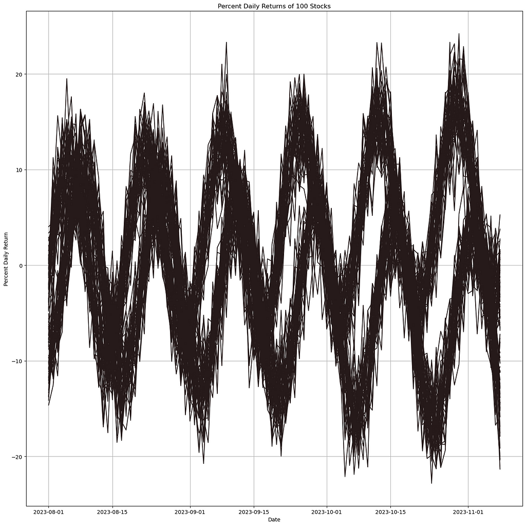
Two Techniques for Visualizing Many Time-Series at Once
Imagine this: you’ve got a bunch of line charts, and you’re confident that there’s at least one trend hiding somewhere in all that data. Whether you’re tracking sales across thousands of your company’s products or diving into stock market data, your goal is to uncover those subtrends and make them stand out in your visualization. Let’s explore a couple of techniques to help you do just that.
Hundreds of lines plotted, but it isn’t clear what the subtrends are. This synthetic data can show the benefit of these strategies. (Image by author)
Option 1 — Density Line Charts:
Density Line Charts are a clever plotting technique introduced by Dominik Moritz and Danyel Fisher in their paper, Visualizing a Million Time Series with the Density Line Chart. This method transforms numerous line charts into heatmaps, revealing areas where the lines overlap the most.
When we apply Density Line Charts to the synthetic data we showed earlier, the results look like this:
PyDLC allows us to see “hot spots” where a high degree of lines overlap. (Image by author)
This implementation allows us to see where our trends are appearing, and identify the subtrends that make this data interesting.
For this example we use the Python library PyDLC by Charles L. Bérubé. The implementation is quite straightforward, thanks to the library’s user-friendly design.
plt.figure(figsize=(14, 14))
im = dense_lines(synth_df.to_numpy().T,
                 x=synth_df.index.astype('int64'),
                 cmap='viridis',
                 ny=100,
                 y_pad=0.01
                )

plt.ylim(-25, 25)

plt.axhline(y=0, color='white', linestyle=':')

plt.show()
When using Density Line Charts, keep in mind that parameters like ny and y_pad may require some tweaking to get the best results.
Option 2— Density Plot of Lines:
This technique isn’t as widely discussed and doesn’t have a universally recognized name. However, it’s essentially a variation of “line density plots” or “line density visualizations,” where we use thicker lines with low opacity to reveal areas of overlap and density.
This technique shows subtrends quite well and reduces cognitive load from the many lines. (Image by author)
We can clearly identify what seem to be two distinct trends and observe the high degree of overlap during the downward movements of the sine waves. However, it’s a bit trickier to pinpoint where the effect is the strongest.
The code for this approach is also quite straightforward:
plt.figure(figsize=(14, 14))

for column in synth_df.columns:
    plt.plot(synth_df.index,
             synth_df[column],
             alpha=0.1,
             linewidth=2,
             label=ticker,
             color='black'
            )
Here, the two parameters that might require some adjustment are alpha and linewidth.
An Example
Imagine we’re searching for subtrends in the daily returns of 50 stocks. The first step is to pull the data and calculate the daily returns.
import yfinance as yf import pandas as pd import numpy as np import matplotlib.pyplot as plt import seaborn as sns
A very messy many-line plot with little discernible information. (Image by author)
The Density Line Chart does face some challenges with this data due to its sporadic nature. However, it still provides valuable insights into overall market trends. For instance, you can spot periods where the densest areas correspond to significant dips, highlighting rough days in the market.
(Image by author)
plt.figure(figsize=(14, 14)) im = dense_lines(pivot_df[stock_tickers].to_numpy().T, x=pivot_df.index.astype('int64'), cmap='viridis', ny=200, y_pad=0.1 )
However, we find that the transparency technique performs significantly better for this particular problem. The market dips we mentioned earlier become much clearer and more discernible.
(Image by author)
plt.figure(figsize=(14, 14))

for ticker in pivot_df.columns:
    plt.plot(pivot_df.index,
             pivot_df[ticker],
             alpha=0.1,
             linewidth=4,
             label=ticker,
             color='black'
            )
Conclusion
Both strategies have their own merits and strengths, and the best approach for your work may not be obvious until you’ve tried both. I hope one of these techniques proves helpful for your future projects. If you have any other techniques or use cases for handling massive line plots, I’d love to hear about them!
Thanks for reading, and take care.
Information in Noise was originally published in Towards Data Science on Medium, where people are continuing the conversation by highlighting and responding to this story.
Customizable R package for Graph / Network visualization
Clinical Flowchart
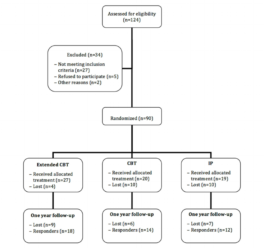
A Clinical (Trial) Flowchart is a visual representation of each step and procedure in a clinical trial or treatment process.
It starts with patients, lists which therapeutic methods are used, which patients are excluded from the trial and for what reason, how the groups are assigned, and so on, and looks like the example below.
Exclude 34 patients due to ineligibility or declining to participate
The remaining 90 patients are randomly assigned to a group (Extended CBT, CBT, IP) to compare treatments.
In each group, 4, 10, and 10 people drop out of the course (although ideally 30 people would be split), and the rest receive the assigned treatment.
When the patients were followed up after 1 year, 9, 6, and 7 were unresponsive, respectively.
The trial started with 124 patients and ended up with only 44 patients, which shows how difficult and expensive clinical trials can be.
Anyway, there is no set way to draw this flowchart, and you can use any commercial software such as PowerPoint or Keynote, or web-based diagramming tools such as draw.io or lucidchart.
Clinical Flowchart with R
I don’t know exactly why, but this time I needed to use R to plot the chart.
The advantages of using a programming approach like R include automation and reuse, integration with other functions (e.g., a program that plots from data source to chart), and a level of customization not available in commercial programs.
Since the original purpose of the package was to draw participant flow diagrams, this is the closest I could get to what I was trying to achieve. I think it’s the best choice unless you have special circumstances.
R package for network visualization graphs based on vis.js.
However, as it turns out, all four methods failed.
This is because there was a special situation with the figure I was trying to draw.
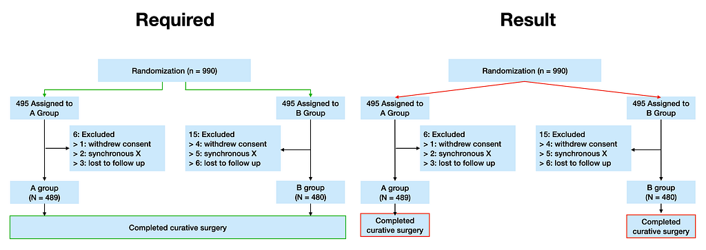
The following figure shows the actual drawing, with only the numbers and groups replaced with 1000, 1,2,3… A, B.
Image by the author
There were two problematic parts: the Completed curative surgery part in the middle, where the two nodes from the previous step connect to one long node, and the difficulty of positioning the edge.
Image by the author
I considered several ways to do this, and eventually decided to use an old friend, shinyCyJS, which I can customize to my purpose.
shinyCyJSis a R package to leverage the network/graph visualization capabilities of cytoscape.js in R. It was the first thing I wrote when I was looking for genomic network visualization when I graduated (at the time, there was only igraph and RCyjs) and didn’t find what I was looking for, which is how I ended up at my current job.
2 Custom feature with shinyCyJS
Positioning Edges
In order to implement the positioning of the edges in the two custom features above, I initially tried to use taxi edges.
However, again, this only determines the edge based on the position of the node, and it is not possible to move the edge, so I switched to adding a microscopic node in the middle and traversing the edge to it, as shown below (since it is possible to specify the position of the “micro” node).
Image by the author
One Big Node
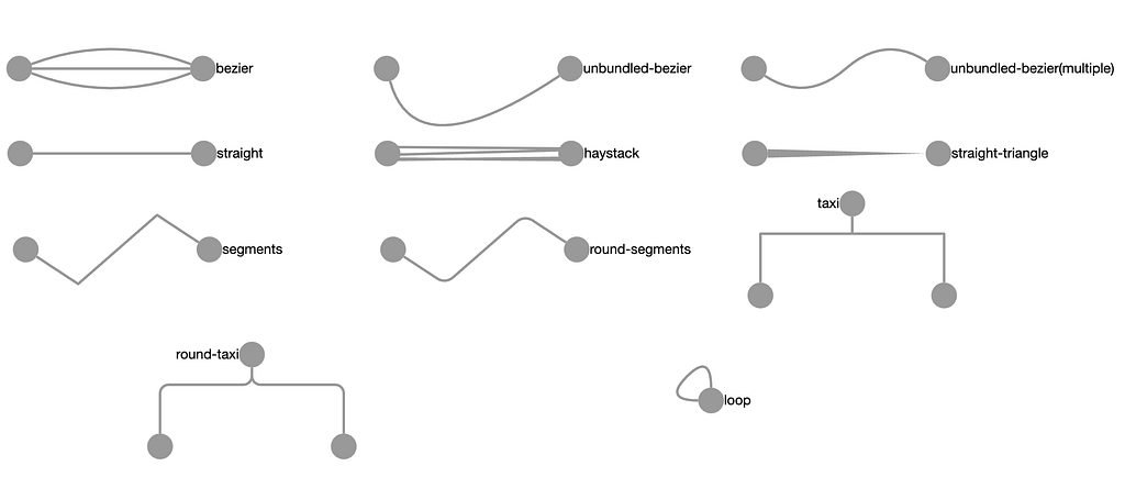
In cytoscape.js, by default, nodes are connected by edges that consider the shortest distance between the center and the center, and if they go through other points along the way, like the taxi mentioned above, the points are not specified and are calculated algorithmically.
The problem with allowing intermediate points to be specified is that when there are multiple edges between nodes, like in the bezier and haystack examples, it is annoying to have to specify intermediate points for all of them.
In the previous example, there are only three edges, so it’s not a big deal, but in the case of genomic networks, which I studied in graduate school, a single gene often interacts with dozens or hundreds of other genes, so it’s a big deal.
In the worst case scenario, the edges overlap and missing a few edges can cause the graph to produce completely different information.
In other words, in the problem of connecting to one long node, the long node is only a graphical (width) perspective for the user,
But from the computer’s point of view, it is irrational behavior to connect an edge to a node that doesn’t even exist, as shown in the image below, so there is no reason to consider this option in the first place.
Image by the author
To solve this problem, I created a micro node and modified it to connect to the appropriate part, just like the previous edge midpoint problem.
Image by the author
Here is a partial view of the graph I ended up creating in R. (Again, groups and numbers are arbitrarily modified)
Image by the author
Another problem, download as PNG
Technically, you can use the Export as PNG button in Rstudio viewer as shown below, and if that doesn’t work, you can take a screenshot, but cytoscape.js has a function to save the graph as png, so I used it.
Image by the author
*I actually had a request to add a download to png feature to shinyCyJS a while back, and I replied “why not just take a screenshot?”.
This required using an internet browser (chrome) (As cytoscape.js is Javascript) and that meant I had to go beyond R and implement it on the web using Shiny.
Of course, shinyCyJS is a package that was built with shiny integration in mind from the start, so it was no problem.
Below is the code you need to run in Chrome’s developer tools to download it
shinyCyJS is an R package I wrote, and it literally does everything cytoscape does, plus custom features like this if needed, so if you need to do network/graph visualization in R, you can try it out or ask for what you need.
Of course, if you don’t need to use R, draw.io seems better.
Additionally, if you want to package other Javascript libraries for use with R, you can send me an email.
The recent successes in AI are often attributed to the emergence and evolutions of the GPU. The GPU’s architecture, which typically includes thousands of multi-processors, high-speed memory, dedicated tensor cores, and more, is particularly well-suited to meet the intensive demands of AI/ML workloads. Unfortunately, the rapid growth in AI development has led to a surge in the demand for GPUs, making them difficult to obtain. As a result, ML developers are increasingly exploring alternative hardware options for training and running their models. In previous posts, we discussed the possibility of training on dedicated AI ASICs such as Google Cloud TPU, Haban Gaudi, and AWS Trainium. While these options offer significant cost-saving opportunities, they do not suit all ML models and can, like the GPU, also suffer from limited availability. In this post we return to the good old-fashioned CPU and revisit its relevance to ML applications. Although CPUs are generally less suited to ML workloads compared to GPUs, they are much easier to acquire. The ability to run (at least some of) our workloads on CPU could have significant implications on development productivity.
In previous posts (e.g., here) we emphasized the importance of analyzing and optimizing the runtime performance of AI/ML workloads as a means of accelerating development and minimizing costs. While this is crucial regardless of the compute engine used, the profiling tools and optimization techniques can vary greatly between platforms. In this post, we will discuss some of the performance optimization options that pertain to CPU. Our focus will be on Intel® Xeon® CPU processors (with Intel® AVX-512) and on the PyTorch (version 2.4) framework (although similar techniques can be applied to other CPUs and frameworks, as well). More specifically, we will run our experiments on an Amazon EC2 c7i instance with an AWS Deep Learning AMI. Please do not view our choice of Cloud platform, CPU version, ML framework, or any other tool or library we should mention, as an endorsement over their alternatives.
Our goal will be to demonstrate that although ML development on CPU may not be our first choice, there are ways to “soften the blow” and — in some cases — perhaps even make it a viable alternative.
Disclaimers
Our intention in this post is to demonstrate just a few of the ML optimization opportunities available on CPU. Contrary to most of the online tutorials on the topic of ML optimization on CPU, we will focus on a training workload rather than an inference workload. There are a number of optimization tools focused specifically on inference that we will not cover (e.g., see here and here).
Please do not view this post as a replacement of the official documentation on any of the tools or techniques that we mention. Keep in mind that given the rapid pace of AI/ML development, some of the content, libraries, and/or instructions that we mention may become outdated by the time you read this. Please be sure to refer to the most-up-to-date documentation available.
Importantly, the impact of the optimizations that we discuss on runtime performance is likely to vary greatly based on the model and the details of the environment (e.g., see the high degree of variance between models on the official PyTorch TouchInductor CPU Inference Performance Dashboard). The comparative performance numbers we will share are specific to the toy model and runtime environment that we will use. Be sure to reevaluate all of the proposed optimizations on your own model and runtime environment.
Lastly, our focus will be solely on throughput performance (as measured in samples per second) — not on training convergence. However, it should be noted that some optimization techniques (e.g., batch size tuning, mixed precision, and more) could have a negative effect on the convergence of certain models. In some cases, this can be overcome through appropriate hyperparameter tuning.
Toy Example — ResNet-50
We will run our experiments on a simple image classification model with a ResNet-50 backbone (from Deep Residual Learning for Image Recognition). We will train the model on a fake dataset. The full training script appears in the code block below (loosely based on this example):
import torch import torchvision from torch.utils.data import Dataset, DataLoader import time
# A dataset with random images and labels class FakeDataset(Dataset): def __len__(self): return 1000000
Running this script on a c7i.2xlarge (with 8 vCPUs) and the CPU version of PyTorch 2.4, results in a throughput of 9.12 samples per second. For the sake of comparison, we note that the throughput of the same (unoptimized script) on an Amazon EC2 g5.2xlarge instance (with 1 GPU and 8 vCPUs) is 340 samples per second. Taking into account the comparative costs of these two instance types ($0.357 per hour for a c7i.2xlarge and $1.212 for a g5.2xlarge, as of the time of this writing), we find that training on the GPU instance to give roughly eleven(!!) times better price performance. Based on these results, the preference for using GPUs to train ML models is very well founded. Let’s assess some of the possibilities for reducing this gap.
PyTorch Performance Optimizations
In this section we will explore some basic methods for increasing the runtime performance of our training workload. Although you may recognize some of these from our post on GPU optimization, it is important to highlight a significant difference between training optimization on CPU and GPU platforms. On GPU platforms much of our effort was dedicated to maximizing the parallelization between (the training data preprocessing on) the CPU and (the model training on) the GPU. On CPU platforms all of the processing occurs on the CPU and our goal will be to allocate its resources most effectively.
Batch Size
Increasing the training batch size can potentially increase performance by reducing the frequency of the model parameter updates. (On GPUs it has the added benefit of reducing the overhead of CPU-GPU transactions such as kernel loading). However, while on GPU we aimed for a batch size that would maximize the utilization of the GPU memory, the same strategy might hurt performance on CPU. For reasons beyond the scope of this post, CPU memory is more complicated and the best approach for discovering the most optimal batch size may be through trial and error. Keep in mind that changing the batch size could affect training convergence.
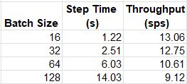
The table below summarizes the throughput of our training workload for a few (arbitrary) choices of batch size:
Training Throughput as Function of Batch Size (by Author)
Contrary to our findings on GPU, on the c7i.2xlarge instance type our model appears to prefer lower batch sizes.
Multi-process Data Loading
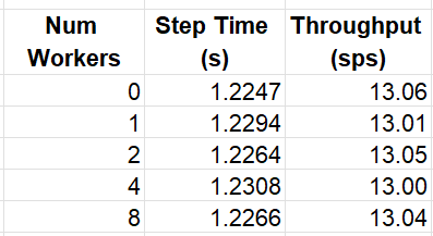
A common technique on GPUs is to assign multiple processes to the data loader so as to reduce the likelihood of starvation of the GPU. On GPU platforms, a general rule of thumb is to set the number of workers according to the number of CPU cores. However, on CPU platforms, where the model training uses the same resources as the data loader, this approach could backfire. Once again, the best approach for choosing the optimal number of workers may be trial and error. The table below shows the average throughput for different choices of num_workers:
Training Throughput as Function of the Number of Data Loading Workers (by Author)
Mixed Precision
Another popular technique is to use lower precision floating point datatypes such as torch.float16 or torch.bfloat16 with the dynamic range of torch.bfloat16 generally considered to be more amiable to ML training. Naturally, reducing the datatype precision can have adverse effects on convergence and should be done carefully. PyTorch comes with torch.amp, an automatic mixed precision package for optimizing the use of these datatypes. Intel® AVX-512 includes support for the bfloat16 datatype. The modified training step appears below:
for idx, (data, target) in enumerate(train_loader):
    optimizer.zero_grad()
    with torch.amp.autocast('cpu',dtype=torch.bfloat16):
        output = model(data)
        loss = criterion(output, target)
    loss.backward()
    optimizer.step()
The throughput following this optimization is 24.34 samples per second, an increase of 86%!!
Channels Last Memory Format
Channels last memory format is a beta-level optimization (at the time of this writing), pertaining primarily to vision models, that supports storing four dimensional (NCHW) tensors in memory such that the channels are the last dimension. This results in all of the data of each pixel being stored together. This optimization pertains primarily to vision models. Considered to be more “friendly to Intel platforms”, this memory format is reported boost the performance of a ResNet-50 on an Intel® Xeon® CPU. The adjusted training step appears below:
for idx, (data, target) in enumerate(train_loader):
    data = data.to(memory_format=torch.channels_last)
    optimizer.zero_grad()
    with torch.amp.autocast('cpu',dtype=torch.bfloat16):
        output = model(data)
        loss = criterion(output, target)
    loss.backward()
    optimizer.step()
The resulting throughput is 37.93 samples per second — an additional 56% improvement and a total of 415% compared to our baseline experiment. We are on a role!!
Torch Compilation
In a previous post we covered the virtues of PyTorch’s support for graph compilation and its potential impact on runtime performance. Contrary to the default eager execution mode in which each operation is run independently (a.k.a., “eagerly”), the compile API converts the model into an intermediate computation graph which is then JIT-compiled into low-level machine code in a manner that is optimal for the underlying training engine. The API supports compilation via different backend libraries and with multiple configuration options. Here we will limit our evaluation to the default (TorchInductor) backend and the ipex backend from the Intel® Extension for PyTorch, a library with dedicated optimizations for Intel hardware. Please see the documentation for appropriate installation and usage instructions. The updated model definition appears below:
import intel_extension_for_pytorch as ipex

model = torchvision.models.resnet50()
backend='inductor' # optionally change to 'ipex'
model = torch.compile(model, backend=backend)
In the case of our toy model, the impact of torch compilation is only apparent when the “channels last” optimization is disabled (and increase of ~27% for each of the backends). When “channels last” is applied, the performance actually drops. As a result, we drop this optimization from our subsequent experiments.
Generally speaking, these kinds of optimizations require a deep level understanding of the CPU architecture and the features of its supporting SW stack. To simplify matters, PyTorch offers the torch.backends.xeon.run_cpu script for automatically configuring the memory and threading libraries so as to optimize runtime performance. The command below will result in the use of the dedicated memory and threading libraries. We will return to the topic of NUMA nodes when we discuss the option of distributed training.
We verify appropriate installation of TCMalloc (conda install conda-forge::gperftools) and Intel’s Open MP library (pip install intel-openmp), and run the following command.
python -m torch.backends.xeon.run_cpu train.py
The use of the run_cpu script further boosts our runtime performance to 39.05 samples per second. Note that the run_cpu script includes many controls for further tuning performance. Be sure to check out the documentation in order to maximize its use.
Combined with the memory and thread optimizations discussed above, the resultant throughput is 40.73 samples per second. (Note that a similar result is reached when disabling the “channels last” configuration.)
Distributed Training on CPU
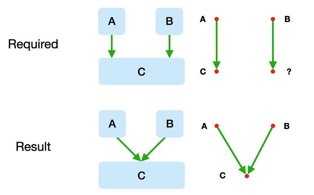
Intel® Xeon® processors are designed with Non-Uniform Memory Access (NUMA) in which the CPU memory is divided into groups, a.k.a., NUMA nodes, and each of the CPU cores is assigned to one node. Although any CPU core can access the memory of any NUMA node, the access to its own node (i.e., its local memory) is much faster. This gives rise to the notion of distributing training across NUMA nodes, where the CPU cores assigned to each NUMA node act as a single process in a distributed process group and data distribution across nodes is managed by Intel® oneCCL, Intel’s dedicated collective communications library.
We can run data distributed training across NUMA nodes easily using the ipexrunutility. In the following code block (loosely based on this example) we adapt our script to run data distributed training (according to usage detailed here):
import os, time import torch from torch.utils.data import Dataset, DataLoader from torch.utils.data.distributed import DistributedSampler import torch.distributed as dist import torchvision import oneccl_bindings_for_pytorch as torch_ccl import intel_extension_for_pytorch as ipex
# configure DDP model = torch.nn.parallel.DistributedDataParallel(model)
# run training loop
# destroy the process group dist.destroy_process_group()
Unfortunately, as of the time of this writing, the Amazon EC2 c7i instance family does not include a multi-NUMA instance type. To test our distributed training script, we revert back to a Amazon EC2 c6i.32xlarge instance with 64 vCPUs and 2 NUMA nodes. We verify the installation of Intel® oneCCL Bindings for PyTorch and run the following command (as documented here):
source $(python -c "import oneccl_bindings_for_pytorch as torch_ccl;print(torch_ccl.cwd)")/env/setvars.sh

# This example command would utilize all the numa sockets of the processor, taking each socket as a rank.
ipexrun cpu --nnodes 1 --omp_runtime intel train.py
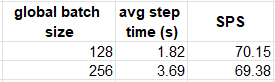
The following table compares the performance results on the c6i.32xlarge instance with and without distributed training:
Distributed Training Across NUMA Nodes (by Author)
In our experiment, data distribution did not boost the runtime performance. Please see ipexrun documentation for additional performance tuning options.
CPU Training with Torch/XLA
In previous posts (e.g., here) we discussed the PyTorch/XLA library and its use of XLA compilation to enable PyTorch based training on XLA devicessuch as TPU, GPU, and CPU. Similar to torch compilation, XLA uses graph compilation to generate machine code that is optimized for the target device. With the establishment of the OpenXLA Project, one of the stated goals was to support high performance across all hardware backends, including CPU (see the CPU RFC here). The code block below demonstrates the adjustments to our original (unoptimized) script required to train using PyTorch/XLA:
model = torchvision.models.resnet50().to(device) criterion = torch.nn.CrossEntropyLoss() optimizer = torch.optim.SGD(model.parameters()) model.train()
for idx, (data, target) in enumerate(train_loader): data = data.to(device) target = target.to(device) optimizer.zero_grad() output = model(data) loss = criterion(output, target) loss.backward() optimizer.step() xm.mark_step()
Unfortunately, (as of the time of this writing) the XLA results on our toy model seem far inferior to the (unoptimized) results we saw above (— by as much as 7X). We expect this to improve as PyTorch/XLA’s CPU support matures.
Results
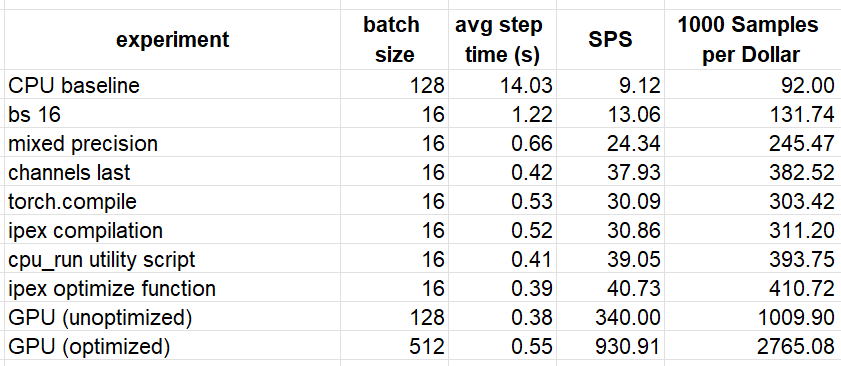
We summarize the results of a subset of our experiments in the table below. For the sake of comparison, we add the throughput of training our model on Amazon EC2 g5.2xlarge GPU instance following the optimization steps discussed in this post. The samples per dollar was calculated based on the Amazon EC2 On-demand pricing page ($0.357 per hour for a c7i.2xlarge and $1.212 for a g5.2xlarge, as of the time of this writing).
Performance Optimization Results (by Author)
Although we succeeded in boosting the training performance of our toy model on the CPU instance by a considerable margin (446%), it remains inferior to the (optimized) performance on the GPU instance. Based on our results, training on GPU would be ~6.7 times cheaper. It is likely that with additional performance tuning and/or applying additional optimizations strategies, we could further close the gap. Once again, we emphasize that the comparative performance results we have reached are unique to this model and runtime environment.
Amazon EC2 Spot Instances Discounts
The increased availability of cloud-based CPU instance types (compared to GPU instance types) may imply greater opportunity for obtaining compute power at discounted rates, e.g., through Spot Instance utilization. Amazon EC2 Spot Instances are instances from surplus cloud service capacity that are offered for a discount of as much as 90% off the On-Demand pricing. In exchange for the discounted price, AWS maintains the right to preempt the instance with little to no warning. Given the high demand for GPUs, you may find CPU spot instances easier to get ahold of than their GPU counterparts. At the time of this writing, c7i.2xlarge Spot Instance price is $0.1291 which would improve our samples per dollar result to 1135.76 and further reduces the gap between the optimized GPU and CPU price performances (to 2.43X).
While the runtime performance results of the optimized CPU training of our toy model (and our chosen environment) were lower than the GPU results, it is likely that the same optimization steps applied to other model architectures (e.g., ones that include components that are not supported by GPU) may result in the CPU performance matching or beating that of the GPU. And even in cases where the performance gap is not bridged, there may very well be cases where the shortage of GPU compute capacity would justify running some of our ML workloads on CPU.
Summary
Given the ubiquity of the CPU, the ability to use them effectively for training and/or running ML workloads could have huge implications on development productivity and on end-product deployment strategy. While the nature of the CPU architecture is less amiable to many ML applications when compared to the GPU, there are many tools and techniques available for boosting its performance — a select few of which we have discussed and demonstrated in this post.
In this post we focused optimizing training on CPU. Please be sure to check out our many other posts on medium covering a wide variety of topics pertaining to performance analysis and optimization of machine learning workloads.
We use cookies on our website to give you the most relevant experience by remembering your preferences and repeat visits. By clicking “Accept”, you consent to the use of ALL the cookies.
This website uses cookies to improve your experience while you navigate through the website. Out of these, the cookies that are categorized as necessary are stored on your browser as they are essential for the working of basic functionalities of the website. We also use third-party cookies that help us analyze and understand how you use this website. These cookies will be stored in your browser only with your consent. You also have the option to opt-out of these cookies. But opting out of some of these cookies may affect your browsing experience.
Necessary cookies are absolutely essential for the website to function properly. These cookies ensure basic functionalities and security features of the website, anonymously.
Cookie
Duration
Description
cookielawinfo-checkbox-analytics
11 months
This cookie is set by GDPR Cookie Consent plugin. The cookie is used to store the user consent for the cookies in the category "Analytics".
cookielawinfo-checkbox-functional
11 months
The cookie is set by GDPR cookie consent to record the user consent for the cookies in the category "Functional".
cookielawinfo-checkbox-necessary
11 months
This cookie is set by GDPR Cookie Consent plugin. The cookies is used to store the user consent for the cookies in the category "Necessary".
cookielawinfo-checkbox-others
11 months
This cookie is set by GDPR Cookie Consent plugin. The cookie is used to store the user consent for the cookies in the category "Other.
cookielawinfo-checkbox-performance
11 months
This cookie is set by GDPR Cookie Consent plugin. The cookie is used to store the user consent for the cookies in the category "Performance".
viewed_cookie_policy
11 months
The cookie is set by the GDPR Cookie Consent plugin and is used to store whether or not user has consented to the use of cookies. It does not store any personal data.
Functional cookies help to perform certain functionalities like sharing the content of the website on social media platforms, collect feedbacks, and other third-party features.
Performance cookies are used to understand and analyze the key performance indexes of the website which helps in delivering a better user experience for the visitors.
Analytical cookies are used to understand how visitors interact with the website. These cookies help provide information on metrics the number of visitors, bounce rate, traffic source, etc.
Advertisement cookies are used to provide visitors with relevant ads and marketing campaigns. These cookies track visitors across websites and collect information to provide customized ads.