Tag: artificial intelligence

A workflow and code walkthrough for building a Bayesian regression model in STAN

Note: Check out my previous article for a practical discussion on why Bayesian modeling may be the right choice for your task.

This tutorial will focus on a workflow + code walkthrough for building a Bayesian regression model in STAN, a probabilistic programming language. STAN is widely adopted and interfaces with your language of choice (R, Python, shell, MATLAB, Julia, Stata). See the installation guide and documentation.

I will use Pystan for this tutorial, simply because I code in Python. Even if you use another language, the general Bayesian practices and STAN language syntax I will discuss here doesn’t vary much.

For the more hands-on reader, here is a link to the notebook for this tutorial, part of my Bayesian modeling workshop at Northwestern University (April, 2024).

Let’s dive in!

Bayesian Linear Regression

Lets learn how to build a simple linear regression model, the bread and butter of any statistician, the Bayesian way. Assuming a dependent variable Y and covariate X, I propose the following simple model-

Y = α + β * X + ϵ

Where ⍺ is the intercept, β is the slope, and ϵ is some random error. Assuming that,

ϵ ~ Normal(0, σ)

we can show that

Y ~ Normal(α + β * X, σ)

We will learn how to code this model form in STAN.

Generate Data

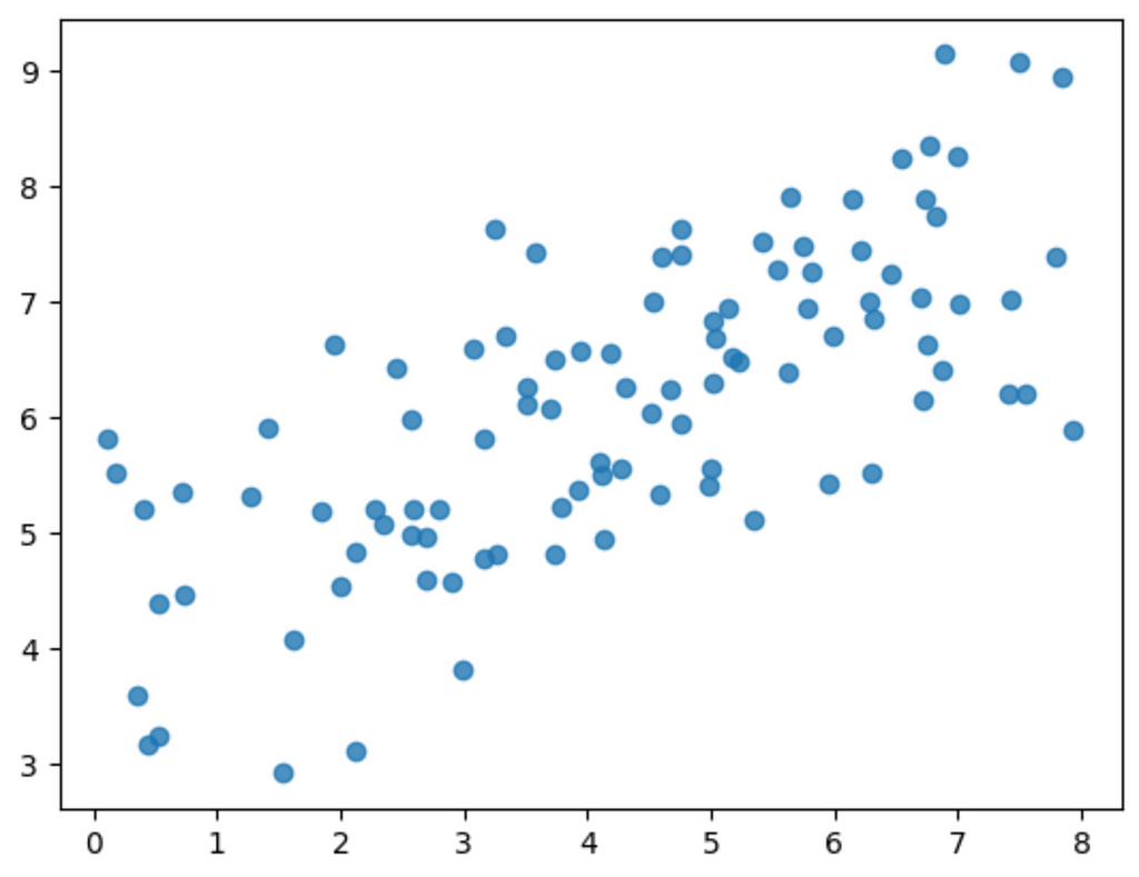
First, let’s generate some fake data.

#Model Parameters
alpha = 4.0  #intercept
beta = 0.5 #slope
sigma = 1.0 #error-scale

#Generate fake data
x =  8 * np.random.rand(100)
y = alpha + beta * x
y = np.random.normal(y, scale=sigma) #noise
#visualize generated data
plt.scatter(x, y, alpha = 0.8)

Model String

Now that we have some data to model, let’s dive into how to structure it and pass it to STAN along with modeling instructions. This is done via the model string, which typically contains 4 (occasionally more) blocks- data, parameters, model, and generated quantities. Let’s discuss each of these blocks in detail.

DATA block

data {                    //input the data to STAN
    int<lower=0> N;
    vector[N] x;
    vector[N] y;
}

The data block is perhaps the simplest, it tells STAN internally what data it should expect, and in what format. For instance, here we pass-

N: the size of our dataset as type int. The <lower=0> part declares that N≥0. (Even though it is obvious here that data length cannot be negative, stating these bounds is good standard practice that can make STAN’s job easier.)

x: the covariate as a vector of length N.

y: the dependent as a vector of length N.

See docs here for a full range of supported data types. STAN offers support for a wide range of types like arrays, vectors, matrices etc. As we saw above, STAN also has support for encoding limits on variables. Encoding limits is recommended! It leads to better specified models and simplifies the probabilistic sampling processes operating under the hood.

Model Block

Next is the model block, where we tell STAN the structure of our model.

//simple model block 
model {                   
    //priors
    alpha ~ normal(0,10);
    beta ~ normal(0,1); 
 
    //model
    y ~ normal(alpha + beta * x, sigma);
}

The model block also contains an important, and often confusing, element: prior specification. Priors are a quintessential part of Bayesian modeling, and must be specified suitably for the sampling task.

See my previous article for a primer on the role and intuition behind priors. To summarize, the prior is a presupposed functional form for the distribution of parameter values — often referred to, simply, as prior belief. Even though priors don’t have to exactly match the final solution, they must allow us to sample from it.

In our example, we use Normal priors of mean 0 with different variances, depending on how sure we are of the supplied mean value: 10 for alpha (very unsure), 1 for beta (somewhat sure). Here, I supplied the general belief that while alpha can take a wide range of different values, the slope is generally more contrained and won’t have a large magnitude.

Hence, in the example above, the prior for alpha is ‘weaker’ than beta.

As models get more complicated, the sampling solution space expands, and supplying beliefs gains importance. Otherwise, if there is no strong intuition, it is good practice to just supply less belief into the model i.e. use a weakly informative prior, and remain flexible to incoming data.

The form for y, which you might have recognized already, is the standard linear regression equation.

Generated Quantities

Lastly, we have our block for generated quantities. Here we tell STAN what quantities we want to calculate and receive as output.

generated quantities {    //get quantities of interest from fitted model
    vector[N] yhat;
    vector[N] log_lik;
    for (n in 1:N){
        yhat[n] = normal_rng(alpha + x[n] * beta, sigma);             
        //generate samples from model
        log_lik[n] = normal_lpdf( y[n] | alpha + x[n] * beta, sigma); 
        //probability of data given the model and parameters
        }
}

Note: STAN supports vectors to be passed either directly into equations, or as iterations 1:N for each element n. In practice, I’ve found this support to change with different versions of STAN, so it is good to try the iterative declaration if the vectorized version fails to compile.

In the above example-

yhat: generates samples for y from the fitted parameter values.

log_lik: generates probability of data given the model and fitted parameter value.

The purpose of these values will be clearer when we talk about model evaluation.

Putting it all together

Altogether, we have now fully specified our first simple Bayesian regression model:

model = """
data {                    //input the data to STAN
    int<lower=0> N;
    vector[N] x;
    vector[N] y;
}

parameters {              
    real alpha;
    real beta;
    real<lower=0> sigma;
}

model {                   
    alpha ~ normal(0,10);
    beta ~ normal(0,1);   
    y ~ normal(alpha + beta * x, sigma);
}

generated quantities {    
    vector[N] yhat;
    vector[N] log_lik;
    
    for (n in 1:N){

        yhat[n] = normal_rng(alpha + x[n] * beta, sigma);             
        log_lik[n] = normal_lpdf(y[n] | alpha + x[n] * beta, sigma);

        }
}
"""

All that remains is to compile the model and run the sampling.

#STAN takes data as a dict
data = {'N': len(x), 'x': x, 'y': y}

STAN takes input data in the form of a dictionary. It is important that this dict contains all the variables that we told STAN to expect in the model-data block, otherwise the model won’t compile.

#parameters for STAN fitting
chains = 2
samples = 1000
warmup = 10
# set seed

# Compile the model
posterior = stan.build(model, data=data, random_seed = 42)
# Train the model and generate samples
fit = posterior.sample(num_chains=chains, num_samples=samples)The .sample() method parameters control the Hamiltonian Monte Carlo (HMC) sampling process, where —

• num_chains: is the number of times we repeat the sampling process.
• num_samples: is the number of samples to be drawn in each chain.
• warmup: is the number of initial samples that we discard (as it takes some time to reach the general vicinity of the solution space).

Knowing the right values for these parameters depends on both the complexity of our model and the resources available.

Higher sampling sizes are of course ideal, yet for an ill-specified model they will prove to be just waste of time and computation. Anecdotally, I’ve had large data models I’ve had to wait a week to finish running, only to find that the model didn’t converge. Is is important to start slowly and sanity check your model before running a full-fledged sampling.

Model Evaluation

The generated quantities are used for

• evaluating the goodness of fit i.e. convergence,
• predictions
• model comparison

Convergence

The first step for evaluating the model, in the Bayesian framework, is visual. We observe the sampling draws of the Hamiltonian Monte Carlo (HMC) sampling process.

In simplistic terms, STAN iteratively draws samples for our parameter values and evaluates them (HMC does way more, but that’s beyond our current scope). For a good fit, the sample draws must converge to some common general area which would, ideally, be the global optima.

The figure above shows the sampling draws for our model across 2 independent chains (red and blue).

• On the left, we plot the overall distribution of the fitted parameter value i.e. the posteriors. We expect a normal distribution if the model, and its parameters, are well specified. (Why is that? Well, a normal distribution just implies that there exist a certain range of best fit values for the parameter, which speaks in support of our chosen model form). Furthermore, we should expect a considerable overlap across chains IF the model is converging to an optima.
• On the right, we plot the actual samples drawn in each iteration (just to be extra sure). Here, again, we wish to see not only a narrow range but also a lot of overlap between the draws.

Not all evaluation metrics are visual. Gelman et al. [1] also propose the Rhat diagnostic which essential is a mathematical measure of the sample similarity across chains. Using Rhat, one can define a cutoff point beyond which the two chains are judged too dissimilar to be converging. The cutoff, however, is hard to define due to the iterative nature of the process, and the variable warmup periods.

Visual comparison is hence a crucial component, regardless of diagnostic tests

A frequentist thought you may have here is that, “well, if all we have is chains and distributions, what is the actual parameter value?” This is exactly the point. The Bayesian formulation only deals in distributions, NOT point estimates with their hard-to-interpret test statistics.

That said, the posterior can still be summarized using credible intervals like the High Density Interval (HDI), which includes all the x% highest probability density points.

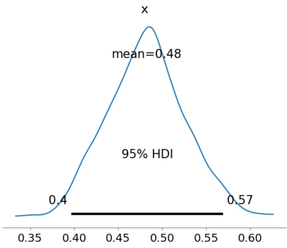
It is important to contrast Bayesian credible intervals with frequentist confidence intervals.

• The credible interval gives a probability distribution on the possible values for the parameter i.e. the probability of the parameter assuming each value in some interval, given the data.
• The confidence interval regards the parameter value as fixed, and estimates instead the confidence that repeated random samplings of the data would match.

Hence the

Bayesian approach lets the parameter values be fluid and takes the data at face value, while the frequentist approach demands that there exists the one true parameter value… if only we had access to all the data ever

Phew. Let that sink in, read it again until it does.

Another important implication of using credible intervals, or in other words, allowing the parameter to be variable, is that the predictions we make capture this uncertainty with transparency, with a certain HDI % informing the best fit line.

Model comparison

In the Bayesian framework, the Watanabe-Akaike Information Metric (WAIC) score is the widely accepted choice for model comparison. A simple explanation of the WAIC score is that it estimates the model likelihood while regularizing for the number of model parameters. In simple words, it can account for overfitting. This is also major draw of the Bayesian framework — one does not necessarily need to hold-out a model validation dataset. Hence,

Bayesian modeling offers a crucial advantage when data is scarce.

The WAIC score is a comparative measure i.e. it only holds meaning when compared across different models that attempt to explain the same underlying data. Thus in practice, one can keep adding more complexity to the model as long as the WAIC increases. If at some point in this process of adding maniacal complexity, the WAIC starts dropping, one can call it a day — any more complexity will not offer an informational advantage in describing the underlying data distribution.

Conclusion

To summarize, the STAN model block is simply a string. It explains to STAN what you are going to give to it (model), what is to be found (parameters), what you think is going on (model), and what it should give you back (generated quantities).

When turned on, STAN simple turns the crank and gives its output.

The real challenge lies in defining a proper model (refer priors), structuring the data appropriately, asking STAN exactly what you need from it, and evaluating the sanity of its output.

Once we have this part down, we can delve into the real power of STAN, where specifying increasingly complicated models becomes just a simple syntactical task. In fact, in our next tutorial we will do exactly this. We will build upon this simple regression example to explore Bayesian Hierarchical models: an industry standard, state-of-the-art, defacto… you name it. We will see how to add group-level radom or fixed effects into our models, and marvel at the ease of adding complexity while maintaining comparability in the Bayesian framework.

Subscribe if this article helped, and to stay-tuned for more!

References

[1] Andrew Gelman, John B. Carlin, Hal S. Stern, David B. Dunson, Aki Vehtari and Donald B. Rubin (2013). Bayesian Data Analysis, Third Edition. Chapman and Hall/CRC.

---

Bayesian Linear Regression: A Complete Beginner’s guide was originally published in Towards Data Science on Medium, where people are continuing the conversation by highlighting and responding to this story.

Yet another LangGraph tutorial

A Task-Oriented Dialogue system (ToD) is a system that assists users in achieving a particular task, such as booking a restaurant, planning a travel itinerary or ordering delivery food.

We know that we instruct LLMs using prompts, but how can we implement these ToD systems so that the conversation always revolves around the task we want the users to achieve? One way of doing that is by using prompts, memory and tool calling. FortunatelyLangChain + LangGraph can help us tie all these things together.

In this article, you’ll learn how to build a Task Oriented Dialogue System that helps users create User Stories with a high level of quality. The system is all based on LangGraph’s Prompt Generation from User Requirements tutorial.

Why do we need to use LangGraph?

In this tutorial we assume you already know how to use LangChain. A User Story has some components like objective, success criteria, plan of execution and deliverables. The user should provide each of them, and we need to “hold their hand” into providing them one by one. Doing that using only LangChain would require a lot of ifs and elses.

With LangGraph we can use a graph abstraction to create cycles to control the dialogue. It also has built-in persistence, so we don’t need to worry about actively tracking the interactions that happen within the graph.

The main LangGraph abstraction is the StateGraph, which is used to create graph workflows. Each graph needs to be initialized with a state_schema: a schema class that each node of the graph uses to read and write information.

The flow of our system will consist of rounds of LLM and user messages. The main loop will contain these steps:

1. User says something
2. LLM reads the messages of the state and decides if it’s ready to create the User Story or if the user should respond again

Our system is simple so the schema consists only of the messages that were exchanged in the dialogue.

from langgraph.graph.message import add_messages

class StateSchema(TypedDict):
    messages: Annotated[list, add_messages]

The add_messages method is used to merge the output messages from each node into the existing list of messages in the graph’s state.

Speaking about nodes, another two main LangGraph concepts are Nodes and Edges. Each node of the graph runs a function and each edge controls the flow of one node to another. We also have START and END virtual nodes to tell the graph where to start the execution and where the execution should end.

To run the system we’ll use the .stream() method. After we build the graph and compile it, each round of interaction will go through the START until the END of the graph and the path it takes (which nodes should run or not) is controlled by our workflow combined with the state of the graph. The following code has the main flow of our system:

config = {"configurable": {"thread_id": str(uuid.uuid4())}}

while True:
    user = input("User (q/Q to quit): ")
    if user in {"q", "Q"}:
        print("AI: Byebye")
        break
    output = None
    for output in graph.stream(
        {"messages": [HumanMessage(content=user)]}, config=config, stream_mode="updates"
    ):
        last_message = next(iter(output.values()))["messages"][-1]
        last_message.pretty_print()

    if output and "prompt" in output:
        print("Done!")

At each interaction (if the user didn’t type “q” or “Q” to quit) we run graph.stream() passing the message of the user using the “updates” stream_mode, which streams the updates of the state after each step of the graph (https://langchain-ai.github.io/langgraph/concepts/low_level/#stream-and-astream). We then get this last message from the state_schema and print it.

In this tutorial we’ll still learn how to create the nodes and edges of the graph, but first let’s talk more about the architecture of ToD systems in general and learn how to implement one with LLMs, prompts and tool calling.

The Architecture of ToD systems

The main components of a framework to build End-to-End Task-Oriented Dialogue systems are [1]:

1. Natural Language Understanding (NLU) for extracting the intent and key slots of users
2. Dialogue State Tracking (DST) for tracing users’ belief state given dialogue
3. Dialogue Policy Learning (DPL) to determine the next step to take
4. Natural Language Generation (NLG) for generating dialogue system response

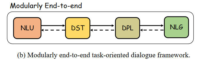
By using LLMs, we can combine some of these components into only one. The NLP and the NLG components are easy peasy to implement using LLMs since understanding and generating dialogue responses are their specialty.

We can implement the Dialogue State Tracking (DST) and the Dialogue Policy Learning (DPL) by using LangChain’s SystemMessage to prime the AI behavior and always pass this message every time we interact with the LLM. The state of the dialogue should also always be passed to the LLM at every interaction with the model. This means that we will make sure the dialogue is always centered around the task we want the user to complete by always telling the LLM what the goal of the dialogue is and how it should behave. We’ll do that first by using a prompt:

prompt_system_task = """Your job is to gather information from the user about the User Story they need to create.

You should obtain the following information from them:

- Objective: the goal of the user story. should be concrete enough to be developed in 2 weeks.
- Success criteria the sucess criteria of the user story
- Plan_of_execution: the plan of execution of the initiative
- Deliverables: the deliverables of the initiative

If you are not able to discern this info, ask them to clarify! Do not attempt to wildly guess. 
Whenever the user responds to one of the criteria, evaluate if it is detailed enough to be a criterion of a User Story. If not, ask questions to help the user better detail the criterion.
Do not overwhelm the user with too many questions at once; ask for the information you need in a way that they do not have to write much in each response. 
Always remind them that if they do not know how to answer something, you can help them.

After you are able to discern all the information, call the relevant tool."""

And then appending this prompt everytime we send a message to the LLM:

def domain_state_tracker(messages):
    return [SystemMessage(content=prompt_system_task)] + messages

Another important concept of our ToD system LLM implementation is tool calling. If you read the last sentence of the prompt_system_task again it says “After you are able to discern all the information, call the relevant tool”. This way, we are telling the LLM that when it decides that the user provided all the User Story parameters, it should call the tool to create the User Story. Our tool for that will be created using a Pydantic model with the User Story parameters.

By using only the prompt and tool calling, we can control our ToD system. Beautiful right? Actually we also need to use the state of the graph to make all this work. Let’s do it in the next section, where we’ll finally build the ToD system.

Creating the dialogue system to build User Stories

Alright, time to do some coding. First we’ll specify which LLM model we’ll use, then set the prompt and bind the tool to generate the User Story:

import os
from dotenv import load_dotenv, find_dotenv

from langchain_openai import AzureChatOpenAI
from langchain_core.pydantic_v1 import BaseModel
from typing import List, Literal, Annotated

_ = load_dotenv(find_dotenv()) # read local .env file

llm = AzureChatOpenAI(azure_deployment=os.environ.get("AZURE_OPENAI_CHAT_DEPLOYMENT_NAME"),
                    openai_api_version="2023-09-01-preview",
                    openai_api_type="azure",
                    openai_api_key=os.environ.get('AZURE_OPENAI_API_KEY'),
                    azure_endpoint=os.environ.get('AZURE_OPENAI_ENDPOINT'),
                    temperature=0)

prompt_system_task = """Your job is to gather information from the user about the User Story they need to create.

You should obtain the following information from them:

- Objective: the goal of the user story. should be concrete enough to be developed in 2 weeks.
- Success criteria the sucess criteria of the user story
- Plan_of_execution: the plan of execution of the initiative

If you are not able to discern this info, ask them to clarify! Do not attempt to wildly guess. 
Whenever the user responds to one of the criteria, evaluate if it is detailed enough to be a criterion of a User Story. If not, ask questions to help the user better detail the criterion.
Do not overwhelm the user with too many questions at once; ask for the information you need in a way that they do not have to write much in each response. 
Always remind them that if they do not know how to answer something, you can help them.

After you are able to discern all the information, call the relevant tool."""

class UserStoryCriteria(BaseModel):
    """Instructions on how to prompt the LLM."""
    objective: str
    success_criteria: str
    plan_of_execution: str

llm_with_tool = llm.bind_tools([UserStoryCriteria])

As we were talking earlier, the state of our graph consists only of the messages exchanged and a flag to know if the user story was created or not. Let’s create the graph first using StateGraph and this schema:

from langgraph.graph import StateGraph, START, END
from langgraph.graph.message import add_messages

class StateSchema(TypedDict):
    messages: Annotated[list, add_messages]
    created_user_story: bool

workflow = StateGraph(StateSchema)

The next image shows the structure of the final graph:

At the top we have a talk_to_user node. This node can either:

• Finalize the dialogue (go to the finalize_dialogue node)
• Decide that it’s time to wait for the user input (go to the END node)

Since the main loop runs forever (while True), every time the graph reaches the END node, it waits for the user input again. This will become more clear when we create the loop.

Let’s create the nodes of the graph, starting with the talk_to_user node. This node needs to keep track of the task (maintaing the main prompt during all the conversation) and also keep the message exchanges because it’s where the state of the dialogue is stored. This state also keeps which parameters of the User Story are already filled or not using the messages. So this node should add the SystemMessage every time and append the new message from the LLM:

def domain_state_tracker(messages):
    return [SystemMessage(content=prompt_system_task)] + messages

def call_llm(state: StateSchema):
    """
    talk_to_user node function, adds the prompt_system_task to the messages,
    calls the LLM and returns the response
    """
    messages = domain_state_tracker(state["messages"])
    response = llm_with_tool.invoke(messages)
    return {"messages": [response]}

Now we can add the talk_to_user node to this graph. We’ll do that by giving it a name and then passing the function we’ve created:

workflow.add_node("talk_to_user", call_llm)

This node should be the first node to run in the graph, so let’s specify that with an edge:

workflow.add_edge(START, "talk_to_user")

So far the graph looks like this:

To control the flow of the graph, we’ll also use the message classes from LangChain. We have four types of messages:

• SystemMessage: message for priming AI behavior
• HumanMessage: message from a human
• AIMessage: the message returned from a chat model as a response to a prompt
• ToolMessage: message containing the result of a tool invocation, used for passing the result of executing a tool back to a model

We’ll use the type of the last message of the graph state to control the flow on the talk_to_user node. If the last message is an AIMessage and it has the tool_calls key, then we’ll go to the finalize_dialogue node because it’s time to create the User Story. Otherwise, we should go to the END node because we’ll restart the loop since it’s time for the user to answer.

The finalize_dialogue node should build the ToolMessage to pass the result to the model. The tool_call_id field is used to associate the tool call request with the tool call response. Let’s create this node and add it to the graph:

def finalize_dialogue(state: StateSchema):
    """
    Add a tool message to the history so the graph can see that it`s time to create the user story
    """
    return {
        "messages": [
            ToolMessage(
                content="Prompt generated!",
                tool_call_id=state["messages"][-1].tool_calls[0]["id"],
            )
        ]
    }

workflow.add_node("finalize_dialogue", finalize_dialogue)

Now let’s create the last node, the create_user_story one. This node will call the LLM using the prompt to create the User Story and the information that was gathered during the conversation. If the model decided that it was time to call the tool then the values of the key tool_calls should have all the info to create the User Story.

prompt_generate_user_story = """Based on the following requirements, write a good user story:

{reqs}"""

def build_prompt_to_generate_user_story(messages: list):
    tool_call = None
    other_msgs = []
    for m in messages:
        if isinstance(m, AIMessage) and m.tool_calls: #tool_calls is from the OpenAI API
            tool_call = m.tool_calls[0]["args"]
        elif isinstance(m, ToolMessage):
            continue
        elif tool_call is not None:
            other_msgs.append(m)
    return [SystemMessage(content=prompt_generate_user_story.format(reqs=tool_call))] + other_msgs


def call_model_to_generate_user_story(state):
    messages = build_prompt_to_generate_user_story(state["messages"])
    response = llm.invoke(messages)
    return {"messages": [response]}

workflow.add_node("create_user_story", call_model_to_generate_user_story)

With all the nodes are created, it’s time to add the edges. We’ll add a conditional edge to the talk_to_user node. Remember that this node can either:

• Finalize the dialogue if it’s time to call the tool (go to the finalize_dialogue node)
• Decide that we need to gather user input (go to the END node)

This means that we’ll only check if the last message is an AIMessage and has the tool_calls key; otherwise we should go to the END node. Let’s create a function to check this and add it as an edge:

def define_next_action(state) -> Literal["finalize_dialogue", END]:
    messages = state["messages"]

    if isinstance(messages[-1], AIMessage) and messages[-1].tool_calls:
        return "finalize_dialogue"
    else:
        return END

workflow.add_conditional_edges("talk_to_user", define_next_action)

Now let’s add the other edges:

workflow.add_edge("finalize_dialogue", "create_user_story")
workflow.add_edge("create_user_story", END)

With that the graph workflow is done. Time to compile the graph and create the loop to run it:

memory = MemorySaver()
graph = workflow.compile(checkpointer=memory)

config = {"configurable": {"thread_id": str(uuid.uuid4())}}

while True:
    user = input("User (q/Q to quit): ")
    if user in {"q", "Q"}:
        print("AI: Byebye")
        break
    output = None
    for output in graph.stream(
        {"messages": [HumanMessage(content=user)]}, config=config, stream_mode="updates"
    ):
        last_message = next(iter(output.values()))["messages"][-1]
        last_message.pretty_print()

    if output and "create_user_story" in output:
        print("User story created!")

Let’s finally test the system:

Final Thoughts

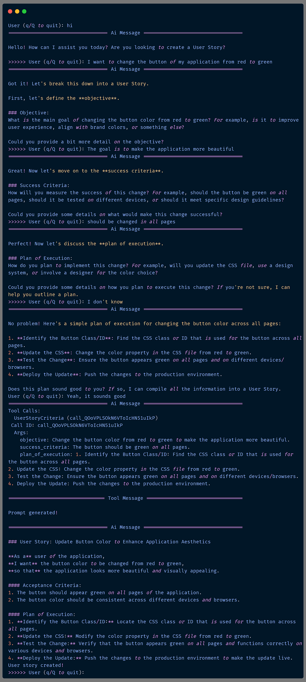
With LangGraph and LangChain we can build systems that guide users through structured interactions reducing the complexity to create them by using the LLMs to help us control the conditional logic.

With the combination of prompts, memory management, and tool calling we can create intuitive and effective dialogue systems, opening new possibilities for user interaction and task automation.

I hope that this tutorial help you better understand how to use LangGraph (I’ve spend a couple of days banging my head on the wall to understand how all the pieces of the library work together).

All the code of this tutorial can be found here: dmesquita/task_oriented_dialogue_system_langgraph (github.com)

Thanks for reading!

References

[1] Qin, Libo, et al. “End-to-end task-oriented dialogue: A survey of tasks, methods, and future directions.” arXiv preprint arXiv:2311.09008 (2023).

[2] Prompt generation from user requirements. Available at: https://langchain-ai.github.io/langgraph/tutorials/chatbots/information-gather-prompting

---

Creating Task-Oriented Dialog systems with LangGraph and LangChain was originally published in Towards Data Science on Medium, where people are continuing the conversation by highlighting and responding to this story.

In this post, we explore a solution that uses generative artificial intelligence (AI) to generate a SQL query from a user’s question in natural language. This solution can simplify the process of querying CUR data stored in an Amazon Athena database using SQL query generation, running the query on Athena, and representing it on a web portal for ease of understanding.