Tag: AI

What happened in 2024 that is new and significant in the world of AI ethics? The new technology developments have come in fast, but what has ethical or values implications that are going to matter long-term?

I’ve been working on updates for my 2025 class on Values and Ethics in Artificial Intelligence. This course is part of the Johns Hopkins Education for Professionals program, part of the Master’s degree in Artificial Intelligence.

Overview of my changes:

I’m doing major updates on three topics based on 2024 developments, and a number of small updates, integrating other news and filling gaps in the course.

Topic 1: LLM interpretability.

Anthropic’s work in interpretability was a breakthrough in explainable AI (XAI). We will be discussing how this method can be used in practice, as well as implications for how we think about AI understanding.

Topic 2: Human-Centered AI.

Rapid AI development adds urgency to the question: How do we design AI to empower rather than replace human beings? I have added content throughout my course on this, including two new design exercises.

Topic 3: AI Law and Governance.

Major developments were the EU’s AI Act and the raft of California legislation, including laws targeting deep fakes, misinformation, intellectual property, medical communications and minor’s use of ‘addictive’ social media, among other. For class I developed some heuristics for evaluating AI legislation, such as studying definitions, and explain how legislation is only one piece of the solution to the AI governance puzzle.

Miscellaneous new material:

I am integrating material from news stories into existing topics on copyright, risk, privacy, safety and social media/ smartphone harms.

Topic 1: Generative AI Interpretability

What’s new:

Anthropic’s pathbreaking 2024 work on interpretability was a fascination of mine. They published a blog post here, and there is also a paper, and there was an interactive feature browser. Most tech-savvy readers should be able to get something out of the blog and paper, despite some technical content and a daunting paper title (‘Scaling Monosemanticity’).

Below is a screenshot of one discovered feature, ‘syncophantic praise’. I like this one because of the psychological subtlety; it amazes me that they could separate this abstract concept from simple ‘flattery’, or ‘praise’.

What’s important:

Explainable AI: For my ethics class, this is most relevant to explainable AI (XAI), which is a key ingredient of human-centered design. The question I will pose to the class is, how might this new capability be used to promote human understanding and empowerment when using LLMs? SAEs (sparse autoencoders) are too expensive and hard to train to be a complete solution to XAI problems, but they can add depth to a multi-pronged XAI strategy.

Safety implications: Anthropic’s work on safety is also worth a mention. They identified the ‘syncophantic praise’ feature as part of their work on safety, specifically relevant to this question: could a very powerful AI hide its intentions from humans, possibly by flattering users into complacency? This general direction is especially salient in light of this recent work: Frontier Models are Capable of In-context Scheming.

Evidence of AI ‘Understanding’? Did interpretability kill the ‘stochastic parrot’? I have been convinced for a while that LLMs must have some internal representations of complex and inter-related concepts. They could not do what they do as one-deep stimulus-response or word-association engines, (‘stochastic parrots’) no matter how many patterns were memorized. The use of complex abstractions, such as those identified by Anthropic, fits my definition of ‘understanding’, although some reserve that term only for human understanding. Perhaps we should just add a qualifier for ‘AI understanding’. This is not a topic that I explicitly cover in my ethics class, but it does come up in discussion of related topics.

SAE visualization needed. I am still looking for a good visual illustration of how complex features across a deep network are mapped onto to a very thin, very wide SAEs with sparsely represented features. What I have now is the Powerpoint approximation I created for class use, below. Props to Brendan Boycroft for his LLM visualizer, which has helped me understand more about the mechanics of LLMs. https://bbycroft.net/llm

Topic 2: Human Centered AI (HCAI)

What’s new?

In 2024 it was increasingly apparent that AI will affect every human endeavor and seems to be doing so at a much faster rate than previous technologies such as steam power or computers. The speed of change matters almost more than the nature of change because human culture, values, and ethics do not usually change quickly. Maladaptive patterns and precedents set now will be increasingly difficult to change later.

What’s important?

Human-Centered AI needs to become more than an academic interest, it needs to become a well-understood and widely practiced set of values, practices and design principles. Some people and organizations that I like, along with the Anthropic explainability work already mentioned, are Stanford’s Human-Centered AI, Google’s People + AI effort, and Ben Schneiderman’s early leadership and community organizing.

For my class of working AI engineers, I am trying to focus on practical and specific design principles. We need to counter the dysfunctional design principles I seem to see everywhere: ‘automate everything as fast as possible’, and ‘hide everything from the users so they can’t mess it up’. I am looking for cases and examples that challenge people to step up and use AI in ways that empower humans to be smarter, wiser and better than ever before.

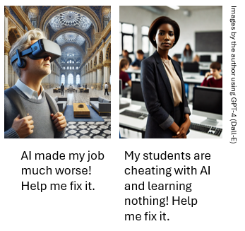
I wrote fictional cases for class modules on the Future of Work, HCAI and Lethal Autonomous Weapons. Case 1 is about a customer-facing LLM system that tried to do too much too fast and cut the expert humans out of the loop. Case 2 is about a high school teacher who figured out most of her students were cheating on a camp application essay with an LLM and wants to use GenAI in a better way.

The cases are on separate Medium pages here and here, and I love feedback! Thanks to Sara Bos and Andrew Taylor for comments already received.

The second case might be controversial; some people argue that it is OK for students to learn to write with AI before learning to write without it. I disagree, but that debate will no doubt continue.

I prefer real-world design cases when possible, but good HCAI cases have been hard to find. My colleague John (Ian) McCulloh recently gave me some great ideas from examples he uses in his class lectures, including the Organ Donation case, an Accenture project that helped doctors and patients make time-sensitive kidney transplant decision quickly and well. Ian teaches in the same program that I do. I hope to work with Ian to turn this into an interactive case for next year.

Topic 3: AI governance

Most people agree that AI development needs to be governed, through laws or by other means, but there’s a lot of disagreement about how.

What’s new?

The EU’s AI Act came into effect, giving a tiered system for AI risk, and prohibiting a list of highest-risk applications including social scoring systems and remote biometric identification. The AI Act joins the EU’s Digital Markets Act and the General Data Protection Regulation, to form the world’s broadest and most comprehensive set of AI-related legislation.

California passed a set of AI governance related laws, which may have national implications, in the same way that California laws on things like the environment have often set precedent. I like this (incomplete) review from the White & Case law firm.

For international comparisons on privacy, I like DLA Piper‘s website Data Protection Laws of the World.

What’s Important?

My class will focus on two things:

1. How we should evaluate new legislation
2. How legislation fits into the larger context of AI governance

How do you evaluate new legislation?

Given the pace of change, the most useful thing I thought I could give my class is a set of heuristics for evaluating new governance structures.

Pay attention to the definitions. Each of the new legal acts faced problems with defining exactly what would be covered; some definitions are probably too narrow (easily bypassed with small changes to the approach), some too broad (inviting abuse) and some may be dated quickly.

California had to solve some difficult definitional problems in order to try to regulate things like ‘Addictive Media’ (see SB-976), ‘AI Generated Media’ (see AB-1836), and to write separate legislation for ‘Generative AI’, (see SB-896). Each of these has some potentially problematic aspects, worthy of class discussion. As one example, The Digital Replicas Act defines AI-generated media as “an engineered or machine-based system that varies in its level of autonomy and that can, for explicit or implicit objectives, infer from the input it receives how to generate outputs that can influence physical or virtual environments.” There’s a lot of room for interpretation here.

Who is covered and what are the penalties? Are the penalties financial or criminal? Are there exceptions for law enforcement or government use? How does it apply across international lines? Does it have a tiered system based on an organization’s size? On the last point, technology regulation often tries to protect startups and small companies with thresholds or tiers for compliance. But California’s governor vetoed SB 1047 on AI safety for exempting small companies, arguing that “Smaller, specialized models may emerge as equally or even more dangerous”. Was this a wise move, or was he just protecting California’s tech giants?

Is it enforceable, flexible, and ‘future-proof’? Technology legislation is very difficult to get right because technology is a fast-moving target. If it is too specific it risks quickly becoming obsolete, or worse, hindering innovations. But the more general or vague it is, the less enforceable it may be, or more easily ‘gamed’. One strategy is to require companies to define their own risks and solutions, which provides flexibility, but will only work if the legislature, the courts and the public later pay attention to what companies actually do. This is a gamble on a well-functioning judiciary and an engaged, empowered citizenry… but democracy always is.

How does legislation fit into the bigger picture of AI governance?

Not every problem can or should be solved with legislation. AI governance is a multi-tiered system. It includes the proliferation of AI frameworks and independent AI guidance documents that go further than legislation should, and provide non-binding, sometimes idealistic goals. A few that I think are important:

• The NIST AI Risk Management Framework. NIST has a good reputation, at least within the federal government, and this framework is being used as the foundation for a lot of other work.
• The Santa Clara Principles, focused on content moderation, has some industry buy-in and specifically calls out government regulators and Mark Zuckerberg for compliance.
• The AI Moratorium addresses the longer-term, existential safety risks. ‘An Overview of AI Catastrophic Risk’ is a good follow-up.
• Professional societies have been active also; IEEE is very involved in publishing standards and has one for Ethically Aligned Design, ACM has a professional Code of Ethics.
• Microsoft Responsible AI Standards is a good example of a corporate AI document with specific requirements, tools and practices.
• Here’s a partial list of many other frameworks

Other miscellaneous topics

Here’s some other news items and topics I am integrating into my class, some of which are new to 2024 and some are not. I will:

• Include a summary of the 2024 bestseller The Anxious Generation, an important synthesis of harms related to social media, smartphones, and associated lifestyle changes. I’m a big fan of Jonathan Haidt’s work.
• Note whether a verdict on the NY Times/ OpenAI case comes out during the semester.
• Mention the cautionary tale of the OnStar/ Lexus-Nexus privacy violation in the module on privacy.
• Work in the issues of AI’s increasing power demands, and the questionable labor practices related to AI content moderators and data labelers.
• Give an assignment on the dangers of synthetic biology, starting with ‘The New Bioweapons’ article from RAND and a (paywalled) article from a Chinese research team, ‘Challenges and recent progress in the governance of biosecurity risks in the era of synthetic biology’, (DOI: 10.1016/j.jobb.2022.02.002). Students can go deeper with a ‘Special Issue on Artificial Intelligence for Synthetic Biology’.
• Include more on LLM-aided misinformation, with good starter articles ‘Combatting Misinformation in the age of LLMs’ and ‘A Survey on the use of Large Language Models (LLMs) in Fake News’. Go deeper with ‘A meta-analysis of correction effects in science-relevant misinformation.’
• Add material on the Content Authenticity Initiative and related C2PA.
• Compare student predictions to the aggregate opinions of ‘Thousands of AI Authors on the Future of AI’, an update on forecasting work that I use every year. If anyone else has a class of students and wants to compare predictions I can send a Qualtrics link.

Thanks for reading! I always appreciate making contact with other people teaching similar courses or with deep knowledge of related areas. And I also always appreciate Claps and Comments!

---

What I’m Updating in My AI Ethics Class for 2025 was originally published in Towards Data Science on Medium, where people are continuing the conversation by highlighting and responding to this story.

The challenges and promises of deep learning for outlier detection, including self-supervised learning techniques

In the last several years, deep-learning approaches have proven to be extremely effective for many machine learning problems, and, not surprisingly, this has included several areas of outlier detection. In fact, for many modalities of data, including image, video, and audio, there’s really no viable option for outlier detection other than deep learning-based methods.

At the same time, though, for tabular and time-series data, more traditional outlier detection methods can still very often be preferable. This is interesting, as deep learning tends to be a very powerful approach to so many problems (and deep learning has been able to solve many problems that are unsolvable using any other method), but tabular data particularly has proven stubbornly difficult to apply deep learning-based methods to, at least in a way that’s consistently competitive with more established outlier detection methods.

In this article (and the next — the second focusses more on self-supervised learning for tabular data), I’ll take a look at why deep learning-based methods tend to work very well for outlier detection for some modalities (looking at image data specifically, but the same ideas apply to video, audio, and some other types of data), and why it can be limited for tabular data.

As well, I’ll cover a couple reasons to nevertheless take a good look at deep learning for tabular outlier detection. One is that the area is moving quickly, holds a great deal of progress, and this is where we’re quite likely to see some of the largest advances in tabular outlier detection in the coming years.

Another is that, while more traditional methods (including statistical tests such as those based on z-scores, interquartile ranges, histograms, and so on, as well as classic machine learning techniques such as Isolation Forests, k-Nearest Neighbors, Local Outlier Factor (LOF), and ECOD), tend to be preferable, there are some exceptions to this, and there are cases even today where deep-learning based approaches can be the best option for tabular outlier detection. We’ll take a look at these as well.

This article continues a series on outlier detection, covering the use of subspaces, PCA, Distance Metric Learning, Shared Nearest Neighbors, Frequent Patterns Outlier Factor, Counts Outlier Detector, and doping.

This article also contains an excerpt from my book, Outlier Detection in Python. That covers image data, and deep learning-based outlier detection, much more thoroughly, but this article provides a good introduction to the main ideas.

Outlier Detection with Image Data

As indicated, with some data modalities, including image data, there are no viable options for outlier detection available today other than deep learning-based methods, so we’ll start by looking at deep learning-based outlier detection for image data.

I’ll assume for this article, you’re reasonably familiar with neural networks and the idea of embeddings. If not, I’d recommend going through some of the many introductory articles online and getting up to speed with that. Unfortunately, I can’t provide that here, but once you have a decent understanding of neural networks and embeddings, you should be good to follow the rest of this.

There are a number of such methods, but all involve deep neural networks in one way or another, and most work by generating embeddings to represent the images.

Some of the most common deep learning-based techniques for outlier detection are based on autoencoders, variational autoencoders (VAEs), and Generative Adversarial Networks (GANs). I’ll cover several approaches to outlier detection in this article, but autoencoders, VAEs, and GANs are a good place to begin.

These are older, well-established ideas and are examples of a common theme in outlier detection: tools or techniques are often developed for one purpose, and later found to be effective for outlier detection. Some of the many other examples include clustering, frequent item sets, Markov models, space-filling curves, and association rules.

Given space constraints, I’ll just go over autoencoders in this article, but will try to cover VAEs, GANs, and some others in future articles. Autoencoders are a form of neural network actually designed originally for compressing data. (Some other compression algorithms are also used on occasion for outlier detection as well.)

As with clustering, frequent item sets, association rules, Markov models, and so on, the idea is: we can use a model of some type to model the data, which then creates a concise summary of the main patterns in the data. For example, we can model the data by describing the clusters (if the data is well-clustered), the frequent item sets in the data, the linear relationships between the features, and so on. With autoencoders, we model the data with a compressed vector representation of the original data.

These models will be able to represent the typical items in the data usually quite well (assuming the models are well-constructed), but often fail to model the outliers well, and so can be used to help identify the outliers. For example, with clustering (i.e., when using a set of clusters to model the data), outliers are the records that don’t fit well into the clusters. With frequent item sets, outliers are the records that contain few frequent items sets. And with autoencoders, outliers are the records that do not compress well.

Where the models are forms of deep neural networks, they have the advantage of being able to represent virtually any type of data, including image. Consequently, autoencoders (and other deep neural networks such as VAEs and GANs) are very important for outlier detection with image data.

Many outlier detectors are also are built using a technique called self-supervised learning (SSL). These techniques are possibly less widely used for outlier detection than autoencoders, VAEs, and GANs, but are very interesting, and worth looking at, at least quickly, as well. I’ll cover these below, but first I’ll take a look at some of the motivations for outlier detection with image data.

Motivations for Outlier Detection with Image Data

One application is with self-driving cars. Cars will have multiple cameras, each detecting one or more objects. The system will then make predictions as to what each object appearing in the images is. One issue faced by these systems is that when an object is detected by a camera, and the system makes a prediction as to what type of object it is, it may predict incorrectly. And further, it may predict incorrectly, but with high confidence; neural networks can be particularly inclined to show high confidence in the best match, even when wrong, making it difficult to determine from the classifier itself if the system should be more cautious about the detected objects. This can happen most readily where the object seen is different from any of the training examples used to train the system.

To address this, outlier detection systems may be run in parallel with the image classification systems, and when used in this way, they’re often specifically looking for items that appear to be outside the distribution of the training data, referred to as out-of-distribution data, OOD.

That is, any vision classification system is trained on some, probably very large, but finite, set of objects. With self-driving cars this may include traffic lights, stop signs, other cars, buses, motorcycles, pedestrians, dogs, fire hydrants, and so on (the model will be trained to recognize each of these classes, being trained on many instances of each). But, no matter how many types of items the system is trained to recognize, there may be other types of (out-of-distribution) object that are encountered when on the roads, and it’s important to determine when the system has encountered an unrecognized object.

This is actually a common theme with outlier detection with image data: we’re very often interested in identifying unusual objects, as opposed to unusual images. That is, things like unusual lighting, colouring, camera angles, blurring, and other properties of the image itself are typically less interesting. Often the background as well, can be distracting from the main goal of identifying unusual items. There are exceptions to this, but this is fairly common, where we are interested really in the nature of the primary object (or a small number of relevant objects) shown in a picture.

Misclassifying objects with self-driving cars can be quite a serious problem — the vehicle may conclude that a novel object (such as a type of vehicle it did not see during training) is an entirely other type of object, likely the closest match visually to any object type that was seen during training. It may, for example, predict the novel vehicle is a billboard, phone pole, or another unmoving object. But if an outlier detector, running in parallel, recognizes that this object is unusual (and likely out-of-distribution, OOD), the system as a whole can adapt a more conservative and cautious approach to the object and any relevant fail-safe mechanisms in place can be activated.

Another common use of outlier detection with image data is in medical imaging, where anything unusual appearing in images may be a concern and worth further investigation. Again, we are not interested in unusual properties of the image itself — only if any of the objects in the images are OOD: unlike anything seen during training (or only rarely seen during training) and therefore rare and possibly an issue.

Other examples are detecting where unusual objects appear in security cameras, or in cameras monitoring industrial processes. Again, anything unusual is likely worth taking note of.

With self-driving cars, detecting OOD objects may allow the team to enhance its training data. With medical imaging or industrial processes, very often anything unusual is a risk of being a problem. And, as with cars, just knowing we’ve detected an OOD object allows the system to be more conservative and not assume the classification predictions are correct.

As detecting OOD objects in images is key to outlier detection in vision, often the training and testing done relates specifically to this. Often with image data, an outlier detection system is trained on images from one data collection, and testing is done using another similar dataset, with the assumption that the images are different enough to be considered to be from a different distribution (and contain different types of object). This, then, tests the ability to detect OOD data.

For example, training may be done using a set of images covering, say, 100 types of bird, with testing done using another set of images of birds. We generally assume that, if different sources for the images are used, any images from the second set will be at least slightly different and may be assumed to be out-of-distribution, though labels may be used to qualify this better as well: if the training set contains, say, European Greenfinch and the test set does as well, it is reasonable to consider these as not OOD.

Autoencoders

To start to look more specifically at how outlier detection can be done with neural networks, we’ll look first at one of the most practical and straightforward methods, autoencoders. There’s more thorough coverage in Outlier Detection in Python, as well as coverage of VAEs, GANs, and the variations of these available in different packages, but this will give some introduction to at least one means to perform outlier detection.

As indicated, autoencoders are a form of neural network that were traditionally used as a compression tool, though they have been found to be useful for outlier detection as well. Auto encoders take input and learn to compress this with as little loss as possible, such that it can be reconstructed to be close to the original. For tabular data, autoencoders are given one row at a time, with the input neurons corresponding to the columns of the table. For image data, they are given one image at a time, with the input neurons corresponding to the pixels of the picture (though images may also be given in an embedding format).

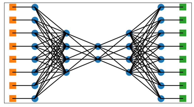
The figure below provides an example of an autoencoder. This is a specific form of a neural network that is designed not to predict a separate target, but to reproduce the input given to the autoencoder. We can see that the network has as many elements for input (the left-most neurons of the network, shown in orange) as for output (the right-most neurons of the network, shown in green), but in between, the layers have fewer neurons. The middle layer has the fewest; this layer represents the embedding (also known as the bottleneck, or the latent representation) for each object.

The size of the middle layer is the size to which we attempt to compress all data, such that it can be recreated (or almost recreated) in the subsequent layers. The embedding created is essentially a concise vector of floating-point numbers that can represent each item.

Autoencoders have two main parts: the first layers of the network are known as the encoder. These layers shrink the data to progressively fewer neurons until they reach the middle of the network. The second part of the network is known as the decoder: a set of layers symmetric with the encoder layers that take the compressed form of each input and attempt to reconstruct it to its original form as closely as possible.

If we are able to train an autoencoder that tends to have low reconstruction error (the output of the network tends to match the input very closely), then if some records have high reconstruction error, they are outliers — they do not follow the general patterns of the data that allow for the compression.

Compression is possible because there are typically some relationships between the features in tabular data, between the words in text, between the concepts in images, and so on. When items are typical, they follow these patterns, and the compression can be quite effective (with minimal loss). When items are atypical, they do not follow these patterns and cannot be compressed without more significant loss.

The number and size of the layers is a modeling decision. The more the data contains patterns (regular associations between the features), the more we are able to compress the data, which means the fewer neurons we can use in the middle layer. It usually takes some experimentation, but we want to set the size of the network so that most records can be constructed with very little, but some, error.

If most records can be recreated with zero error, the network likely has too much capacity — the middle layer is able to fully describe the objects being passed through. We want any unusual records to have a larger reconstruction error, but also to be able to compare this to the moderate error we have with typical records; it’s hard to gauge how unusual a record’s reconstruction error is if almost all other records have an error of 0.0. If this occurs, we know we need to scale back the capacity of the model (reduce the number or neurons) until this is no longer possible. This can, in fact, be a practical means to tune the autoencoder — starting with, for example, many neurons in the middle layers and then gradually adjusting the parameters until you get the results you want.

In this way, autoencoders are able to create an embedding (compressed form of the item) for each object, but we typically do not use the embedding outside of this autoencoder; the outlier scores are usually based entirely on the reconstruction error.

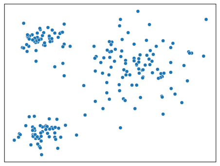
This is not always the case though. The embeddings created in the middle layer are legitimate representations of the objects and can be used for outlier detection. The figure below shows an example where we use two neurons for the middle layer, which allows plotting the latent space as a scatter plot. The x dimension represents the values appearing in one neuron and the y dimension in the other neuron. Each point represents the embedding of an object (possibly an image, sound clip, document, or a table row).

Any standard outlier detector (e.g. KNN, Isolation Forest, Convex Hull, Mahalanobis distance, etc.) can then be used on the latent space. This provides an outlier detection system that is somewhat interpretable if limited to two or three dimensions, but, as with principal component analysis (PCA) and other dimensionality reduction methods, the latent space itself is not interpretable.

Assuming we use the reconstruction error to identify outliers, to calculate the error, any distance metric may be used to measure the distance between the input vector and the output vector. Often Cosine, Euclidean or Manhattan distances are used, with a number of others being fairly common as well. In most cases, it is best to standardize the data before performing outlier detection, both to allow the neural network to fit better and to measure the reconstruction error more fairly. Given this, the outlier score of each record can be calculated as the reconstruction error divided by the median reconstruction error (for some reference dataset).

Another approach, which can be more robust, is to not use a single error metric for the reconstruction, but to use several. This allows us to effectively use the autoencoder to generate a set of features for each record (each relating to a measurement of the reconstruction error) and pass this to a standard outlier detection tool, which will find the records with unusually large values given by one or more reconstruction error metrics.

In general, autoencoders can be an effective means to locate outliers in data, even where there are many features and the outliers are complex — for example with tabular data, spanning many features. One challenge of autoencoders is they do require setting the architecture (the number of layers of the network and the number of neurons per layer), as well as many parameters related to the network (the activation method, learning rate, dropout rate, and so on), which can be difficult to do.

Any model based on neural networks will necessarily be more finicky to tune than other models. Another limitation of AEs is they may not be appropriate with all types of outlier detection. For example, with image data, they will measure the reconstruction at the pixel level (at least if pixels are used as the input), which may not always be relevant.

Interestingly, GANs can perform better in this regard. The general approach to apply GANs to outlier detection is in some ways similar, but a little more involved. The main idea here, though, is that such deep networks can be used effectively for outlier detection, and that they work similarly for any modality of data, though different detectors will flag different types of outliers, and these may be of more or less interest than other outliers.

Self-supervised Learning for Image Data

As indicated, self-supervised learning (SSL) is another technique for outlier detection with image data (and all other types of data), and is also worth taking a look at.

You’re possibly familiar SSL already if you’re used to working with deep learning in other contexts. It’s quite standard for most areas of deep learning, including where the large neural networks are ultimately used for classification, regression, generation, or other tasks. And, if you’re familiar at all with large language models, you’re likely familiar with the idea of masking words within a piece of text and training a neural network to guess the masked word, which is a form of SSL.

The idea, when working with images, is that we often have a very large collection of images, or can easily acquire a large collection online. In practice we would normally actually simply use a foundation model that has itself been trained in a self-supervised manner, but in principle we can do this ourselves, and in any case, what we’ll describe here is roughly what the teams creating the foundation models do.

Once we have a large collection of images, these are almost certainly unlabeled, which means they can’t immediately be used to train a model (training a model requires defining some loss function, which requires a ground truth label for each item). We’ll need to assign labels to each of the images in one way or another. One way is to manually label the data, but this is expensive, time-consuming, and error-prone. It’s also possible to use self-supervised learning, and much of the time this is much more practical.

With SSL, we find a way to arrange the data such that it can automatically be labelled in some way. As indicated, masking is one such way, and is very common when training large language models, and the same masking technique can be used with image data. With images, instead of masking a word, we can mask an area of an image (as in the image of a mug below), and train a neural network to guess the content of the masked out areas.

With image data, several other techniques for self-supervised learning are possible as well.

In general, they work on the principle of creating what’s called a proxy task or a pretext task. That is, we train a model to predict something (such as the missing areas of an image) on the pretext that this is what we are interested in, though in fact our goal actually to train a neural network that understands the images. We can also say, the task is a proxy for this goal.

This is important, as there’s no way to specifically train for outlier detection; proxy tasks are necessary. Using these, we can create a foundation model that has a good general understand of images (a good enough understanding that it is able to perform the proxy task). Much like foundation models for language, these models can then be fine-tuned to be used for other tasks. This can include classification, regression and other such tasks, but also outlier detection.

That is, training in this way (creating a label using self-supervised learning, and training on a proxy task to predict this label), can create a strong foundation model — in order to perform the proxy task (for example, estimating the content of the masked areas of the image), it needs to have a strong understanding of the type of images it’s working with. Which also means, it may be well set up to identify anomalies in the images.

The trick with SSL for outlier detection is to identify good proxy tasks, that allow us to create a good representation of the domain we are modelling, and that allows us to reliably identify any meaningful anomalies in the data we have.

With image data, there are many opportunities to define useful pretext tasks. We have a large advantage that we don’t have with many other modalities: if we have a picture of an object, and we distort the image in any way, it’s still an image of that same object. And, as indicated, it’s most often the object that we’re interested in, not the picture. This allows us to perform many operations on the images that can support, even if indirectly, our final goal of outlier detection.

Some of these include: rotating the image, adjusting the colours, cropping, and stretching, along with other such perturbations of the images. After performing these transformations, the image may look quite different, and at the pixel level, it is quite different, but the object that is shown is the same.

This opens up at least a couple of methods for outlier detection. One is to take advantage of these transformations to create embeddings for the images and identify the outliers as those with unusual embeddings. Another is to use the transformations more directly. I’ll describe both of these in the next sections.

Creating embeddings and using feature modeling

There are quite a number of ways to create embeddings for images that may be useful for outlier detection. I’ll describe one here called contrastive learning.

This takes advantage of the fact that perturbed versions of the same image will represent the same object and so should have similar embeddings. Given that, we can train a neural network to, given two or more variations of the same image, give these similar embeddings, while assigning different embeddings to different images. This encourages the neural network to focus on the main object in each image and not the image itself, and to be robust to changes in colour, orientation, size, and so on.

But, contrastive learning is merely one means to create embeddings for images, and many others, including any self-supervised means, may work best for any given outlier detection task.

Once we have embeddings for the images, we can identify the objects with unusual embeddings, which will be the embeddings unusually far from most other embeddings. For this, we can use the Euclidean, cosine, or other distance measures between the images in the embedding space.

An example of this with tabular data is covered in the next article in this series.

Using the pretext tasks directly

What can also be interesting and quite effective is to use the perturbations more directly to identify the outliers. As an example, consider rotating an image.

Given an image, we can rotate it 0, 90, 180, and 270 degrees, and so then have four versions of the same image. We can then train a neural network to predict, given any image, if it was rotated 0, 90, 180, or 270 degrees. As with some of the examples above (where outliers may be items that do not fit into clusters well, do not contain the frequent item patterns, do not compress well, and so on), here outliers are the images where the neural network cannot predict well how much each version of the image was rotated.

With typical images, when we pass the four variations of the image through the network (assuming the network was well-trained), it will tend to predict the rotation of each of these correctly, but with atypical images, it will not be able to predict accurately, or will have lower confidence in the predictions.

The same general approach can be used with other perturbations, including flipping the image, zooming in, stretching, and so on — in these examples the model predicts how the image was flipped, the scale of the image, or how it was stretched.

Some of these may be used for other modalities as well. Masking, for example, may be used with virtually any modality. Some though, are not as generally applicable; flipping, for example, may not be effective with audio data.

Techniques for outlier detection with image data

I’ll recap here what some of the most common options are:

• Autoencoders, variational autoencoders, and Generative Adversarial networks. These are well-established and quite likely among the most common methods for outlier detection.
• Feature modeling — Here embeddings are created for each object and standard outlier detection (e.g., Isolation Forest, Local Outlier Factor (LOF), k-Nearest Neighbors (KNN), or a similar algorithm) is used on the embeddings. As discussed in the next article, embeddings created to support classification or regression problems do not typically tend to work well in this situation, but we look later at some research related to creating embeddings that are more suitable for outlier detection.
• Using the pretext tasks directly. For example, predicting the rotation, stretching, scaling, etc. of an image. This is an interesting approach, and may be among the most useful for outlier detection.
• Confidence scores — Here we consider where a classifier is used, and the confidence associated with all classes is low. If a classifier was trained to identify, say, 100 types of birds, then it will, when presented with a new image, generate a probability for each of those 100 types of bird. If the probability for all these is very low, the object is unusual in some way and quite likely out of distribution. As indicated, classifiers often provide high confidences even when incorrect, and so this method isn’t always reliable, but even where it is not, when low confidence scores are returned, a system can take advantage of this and recognize that the image is unusual in some regard.

Neural networks with image data

With image data, we are well-positioned to take advantage of deep neural networks, which can create very sophisticated models of the data: we have access to an extremely large body of data, we can use tools such as autoencoders, VAEs and GANS, and self-supervised learning is quite feasible.

One of the important properties of deep neural networks is that they can be grown to very large sizes, which allows them to take advantage of additional data and create even more sophisticated models.

This is in distinction from more traditional outlier detection models, such as Frequent Patterns Outlier Factor (FPOF), association rules, k-Nearest Neighbors, Isolation Forest, LOF, Radius, and so on: as they train on additional data, they may develop slightly more accurate models of normal data, but they tend to level off after some time, with greatly diminishing returns from training with additional data beyond some point. Deep learning models, on the other hand, tend to continue to take advantage of access to more data, even after huge amounts of data have already been used.

We should note, though, that although there has been a great deal of progress in outlier detection with images, it is not yet a solved problem. It is much less subjective than with other modalities, at least where it is defined to deal strictly with out-of-distribution data (though it is still somewhat vague when an object really is of a different type than the objects seen during training — for example, with birds, if a Jay and a Blue Jay are distinct categories). Image data is challenging to work with, and outlier detection is still a challenging area.

Tools for deep learning-based outlier detection

There are several tools that may be used for deep learning-based outlier detection. Three of these, which we’ll look at here and in the next article, are are PyOD, DeepOD, and Alibi-Detect.

PyOD, I’ve covered in some previous articles, and is likely the most comprehensive tool available today for outlier detection on tabular data in python. It contains several standard outlier detectors (Isolation Forest, Local Outlier Factor, Kernel Density Estimation (KDE), Histogram-Based Outlier-Detection (HBOS), Gaussian Mixture Models (GMM), and several others), as well as a number of deep learning-based models, based on autoencoders, variation autoencoders, GANS, and variations of these.

DeepOD provides outlier detection for tabular and time series data. I’ll take a closer look at this in the next article.

Alibi-Detect covers outlier detection for tabular, time-series, and image data. An example of this with image data is shown below.

Most deep learning work today is based on either TensorFlow/Keras or PyTorch (with PyTorch gaining an increasingly large share). Similarly, most deep learning-based outlier detection uses one or the other of these.

PyOD is probably the most straight-forward of these three libraries, at least in my experience, but all are quite manageable and well-documented.

Example using PyOD

This section shows an example using PyOD’s AutoEncoder outlier detector for a tabular dataset (specifically the KDD dataset, available with a public license).

Before using PyOD, it’s necessary to install it, which may be done with:

pip install pyod

You’ll then need to install either TensorFlow or PyTorch if they’re not already installed (depending which detector is being used). I used Google colab for this, which has both TensorFlow & PyTorch installed already. This example uses PyOD’s AutoEncoder outlier detector, which uses PyTorch under the hood.

import pandas as pd
import numpy as np
from sklearn.datasets import fetch_kddcup99
from pyod.models.auto_encoder import AutoEncoder

# Load the data
X, y = fetch_kddcup99(subset="SA", percent10=True, random_state=42, 
                      return_X_y=True, as_frame=True)

# Convert categorical columns to numeric, using one-hot encoding
cat_columns = ["protocol_type", "service", "flag"]
X = pd.get_dummies(X, columns=cat_columns)

det = AutoEncoder()
det.fit(X)
scores = det.decision_scores_

Although an autoencoder is more complicated than many of the other detectors supported by PyOD (for example, HBOS is based in histograms, Cook’s Distance on linear regression; some others are also relatively simple), the interface to work with the autoencoder detector in PyOD is just as simple. This is especially true where, as in this example, we use the default parameters. The same is true for detectors provided by PyOD based on VAEs and GANs, which are, under the hood, even a little more complex than autoencoders, but the API, other than the parameters, is the same.

In this example, we simply load in the data, convert the categorical columns to numeric format (this is necessary for any neural-network model), create an AutoEncoder detector, fit the data, and evaluate each record in the data.

Alibi-Detect

Alibi-Detect also supports autoencoders for outlier detection. It does require some more coding when creating detectors than PyOD; this can be slightly more work, but also allows more flexibility. Alibi-Detect’s documentation provides several examples, which are useful to get you started.

The listing below provides one example, which can help explain the general idea, but it is best to read through their documentation and examples to get a thorough understanding of the process. The listing also uses an autoencoder outlier detector. As alibi-detect can support image data, we provide an example using this.

Working with deep neural networks can be slow. For this, I’d recommend using GPUs if possible. For example, some of the examples found on Alibi-Detect’s documentation, or variations on these I’ve tested, may take about 1 hour on Google colab using a CPU runtime, but only about 3 minutes using the T4 GPU runtime.

Example of Outlier Detection for Image Data

For this example, I just provide some generic code that can be used for any dataset, though the dimensions of the layers will have to be adjusted to match the size of the images used. This example just calls a undefined method called load_data() to get the relevant data (the next example looks closer at specific dataset — here I’m just showing the general system Alibi-Detect uses).

This example starts by first using Keras (if you’re more familiar with PyTorch, the ideas are similar when using Keras) to create the encoder and decoders used by the autoencoder, and then passing these as parameters to the OutlierAE object alibi-detect provides.

As is common with image data, the neural network includes convolutional layers. These are used at times with other types of data as well, including text and time series, though rarely with tabular. It also uses a dense layer.

The code assumes the images are 32×32. With other sizes, the decoder must be organized so that it outputs images of this size as well. The OutlierAE class works by comparing the input images to the the output images (after passing the input images through both the encoder and decoder), so the output images must have identical sizes as the input. This is a bit more finicky when using Conv2D and Conv2DTranspose layers, as in this example, than when using dense layers.

We then call fit() and predict(). For fit(), we specify five epochs. Using more may work better but will also require more time. Alibi-detect’s OutlierAE uses the reconstruction error (specifically, the mean squared error of the reconstructed image from the original image).

import matplotlib.pyplot as plt
import numpy as np
import tensorflow as tf
tf.keras.backend.clear_session()
from tensorflow.keras.layers import Conv2D, Conv2DTranspose, 
    Dense, Layer, Reshape, InputLayer, Flatten
from alibi_detect.od import OutlierAE

# Loads the data used
train, test = load_data() 

X_train, y_train = train
X_test, y_test = test
X_train = X_train.astype('float32') / 255
X_test = X_test.astype('float32') / 255

encoding_dim = 1024

# Defines the encoder portion of the AE
encoder_net = tf.keras.Sequential([ 
      InputLayer(input_shape=(32, 32, 3)),
      Conv2D(64, 4, strides=2, padding='same', activation=tf.nn.relu),
      Conv2D(128, 4, strides=2, padding='same', activation=tf.nn.relu),
      Conv2D(512, 4, strides=2, padding='same', activation=tf.nn.relu),
      Flatten(),
      Dense(encoding_dim,)])

# Defines the decoder portion of the AE
decoder_net = tf.keras.Sequential([ 
      InputLayer(input_shape=(encoding_dim,)),
      Dense(4*4*128),
      Reshape(target_shape=(4, 4, 128)),
      Conv2DTranspose(256, 4, strides=2, padding='same',
          activation=tf.nn.relu),
      Conv2DTranspose(64, 4, strides=2, padding='same', 
          activation=tf.nn.relu),
      Conv2DTranspose(3, 4, strides=2, padding='same', 
          activation='sigmoid')])

# Specifies the threshold for outlier scores
od = OutlierAE(threshold=.015,  
               encoder_net=encoder_net,  
               decoder_net=decoder_net)
od.fit(X_train, epochs=5, verbose=True)

# Makes predictions on the records
X = X_train
od_preds = od.predict(X,
                      outlier_type='instance',    
                      return_feature_score=True,  
                      return_instance_score=True)
print("Number of outliers with normal data:",  
   od_preds['data']['is_outlier'].tolist().count(1))

This makes predictions on the rows used from the training data. Ideally, none are outliers.

Example using PyTorch

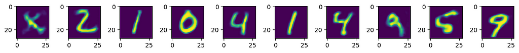
As autoencoders are fairly straightforward to create, this is often done directly, as well as with tools such as Alibi-Detect or PyOD. In this example we work with the MNIST dataset (available with a public license, in this case distributed with PyTorch’s torchvision) and show a quick example using PyTorch.

import numpy as np
import torch
from torchvision import datasets, transforms
from matplotlib import pyplot as plt
import torch.nn as nn
import torch.nn.functional as F
import torch.optim as optim
from torchvision.utils import make_grid

# Collect the data
train_dataset = datasets.MNIST(root='./mnist_data/', train=True, 
  transform=transforms.ToTensor(), download=True)
test_dataset = datasets.MNIST(root='./mnist_data/', train=False, 
  transform=transforms.ToTensor(), download=True)

# Define DataLoaders
batchSize=128
train_loader = torch.utils.data.DataLoader(dataset=train_dataset, batch_size=batchSize, shuffle=True) 
test_loader = torch.utils.data.DataLoader(dataset=test_dataset, batch_size=batchSize, shuffle=False)  

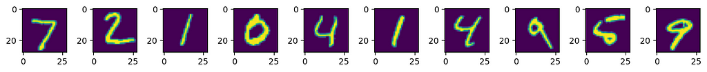
# Display a sample of the data
inputs, _ = next(iter(test_loader))
fig, ax = plt.subplots(nrows=1, ncols=10, figsize=(12, 4))
for i in range(10):
  ax[i].imshow(inputs[i][0])
plt.tight_layout()
plt.show()

# Define the properties of the autoencoder
num_input_pixels = 784  
num_neurons_1 = 256  
num_neurons_2 = 64   

# Define the Autoencoder
class Autoencoder(nn.Module):
    def __init__(self, x_dim, h_dim1, h_dim2):
        super(Autoencoder, self).__init__()
        
        # Encoder
        self.layer1 = nn.Linear(x_dim, h_dim1)
        self.layer2 = nn.Linear(h_dim1, h_dim2)

        # Decoder
        self.layer3 = nn.Linear(h_dim2, h_dim1)
        self.layer4 = nn.Linear(h_dim1, x_dim)

    def encoder(self, x):
        x = torch.sigmoid(self.layer1(x))
        x = torch.sigmoid(self.layer2(x))
        return x

    def decoder(self, x):
        x = torch.sigmoid(self.layer3(x))
        x = torch.sigmoid(self.layer4(x))
        return x

    def forward(self, x):
        x = self.encoder(x)
        x = self.decoder(x)
        return x

model = Autoencoder(num_input_pixels, num_neurons_1, num_neurons_2)
model.cuda()

optimizer = optim.Adam(model.parameters())
n_epoch = 20
loss_function = nn.MSELoss()

for i in range(n_epoch):
    train_loss = 0
    for batch_idx, (data, _) in enumerate(train_loader):
        data = data.cuda()        
        inputs = torch.reshape(data,(-1, 784)) 
        optimizer.zero_grad()

        # Get the result of passing the input through the network      
        recon_x = model(inputs)        

        # The loss is in terms of the difference between the input and
        # output of the model
        loss = loss_function(recon_x, inputs)        
        loss.backward()
        train_loss += loss.item()
        optimizer.step()
        
    if i % 5 == 0:    
        print(f'Epoch: {i:>3d} Average loss: {train_loss:.4f}')
print('Training complete...')

This example uses cuda, but this can be removed where no GPU is available.

In this example, we collect the data, create a DataLoader for the train and for the test data (this is done with most projects using PyTorch), and show a sample of the data, which we see here:

The data contains hand-written digits.

We next define an autoencoder, which defines the encoder and decoder both clearly. Any data passed through the autoencoder goes through both of these.

The autoencoder is trained in a manner similar to most neural networks in PyTorch. We define an optimizer and loss function, and iterate over the data for a certain number of epochs (here using 20), each time covering the data in some number of batches (this uses a batch size of 128, so 16 batches per epoch, given the full data size). After each batch, we calculate the loss, which is based on the difference between the input and output vectors, then update the weights, and continue.

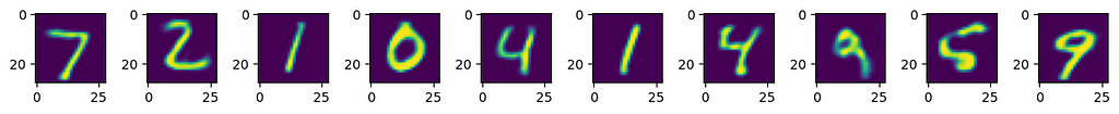
Executing the following code, we can see that with most digits, the reconstruction error is very small:

inputs, _ = next(iter(test_loader))

fig, ax = plt.subplots(nrows=1, ncols=10, figsize=(12, 4))
for i in range(10):
  ax[i].imshow(inputs[i][0])
plt.tight_layout()
plt.show()

inputs=inputs.cuda()
inputs=torch.reshape(inputs,(-1,784))
outputs=model(inputs)
outputs=torch.reshape(outputs,(-1,1,28,28))
outputs=outputs.detach().cpu()

fig, ax = plt.subplots(nrows=1, ncols=10, figsize=(12, 4))
for i in range(10):
  ax[i].imshow(outputs[i][0])
plt.tight_layout()
plt.show()

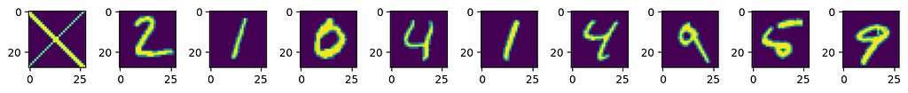
We can then test with out-of-distribution data, passing in this example a character close to an X (so unlike any of the 10 digits it was trained on).

inputs, _ = next(iter(test_loader))

for i in range(28):
  for j in range(28):
    inputs[0][0][i][j] = 0
    if i == j:
      inputs[0][0][i][j] = 1
    if i == j+1:
      inputs[0][0][i][j] = 1
    if i == j+2:
      inputs[0][0][i][j] = 1
    if j == 27-i:
      inputs[0][0][i][j] = 1

fig, ax = plt.subplots(nrows=1, ncols=10, figsize=(12, 4))
for i in range(10):
  ax[i].imshow(inputs[i][0])
plt.tight_layout()
plt.show()

inputs=inputs.cuda()
inputs=torch.reshape(inputs,(-1,784))
outputs=model(inputs)
outputs=torch.reshape(outputs,(-1,1,28,28))
outputs=outputs.detach().cpu()

fig, ax = plt.subplots(nrows=1, ncols=10, figsize=(12, 4))
for i in range(10):
  ax[i].imshow(outputs[i][0])
plt.tight_layout()
plt.show()   

This outputs:

In this case, we see that the reconstruction error for the X is not huge — it’s able to recreate what looks like an X, but the error is unusually large relative to the other characters.

Deep learning-based outlier detection with tabular data

In order to keep this article a manageable length, I’ll wrap up here and continue with tabular data in the next article. For now I’ll just recap that the methods above (or variations of them) can be applied to tabular data, but that there are some significant differences with tabular data that make these techniques more difficult. For example, it’s difficult to create embeddings to represent table records that are more effective for outlier detection than simply using the original records.

As well, the transformations that may be applied to images do not tend to lend themselves well to table records. When perturbing an image of a given object, we can be confident that the new image is still an image of the same object, but when we perturb a table record (especially without strong domain knowledge), we cannot be confident that it’s semantically the same before and after the perturbation. We will, though, look in the next article at techniques to work with tabular data that is often quite effective, and some of the tools available for this.

I’ll also go over, in the next article, challenges with using embeddings for outlier detection, and techniques to make them more practical.

Conclusions

Deep learning is necessary for outlier detection with many modalities including image data, and is showing promise for other areas where it is not yet as well-established, such as tabular data. At present, however, more traditional outlier detection methods still tend to work best for tabular data.

Having said that, there are cases now where deep learning-based outlier detection can be the most effective method for identifying anomalies in tabular data, or at least can be useful to include among the methods examined (and possibly included in a larger ensemble of detectors).

There are many approaches to using deep learning for outlier detection, and we’ll probably see more developed in coming years. Some of the most established are autoencoders, variational autoencoders, and GANs, and there is good support for these in the major outlier detection libraries, including PyOD and Alibi-Detect.

Self-supervised learning for outlier detection is also showing a great deal of promise. We’ve covered here how it can be applied to image data, and cover tabular data in the next article. It can, as well, be applied, in one form or another, to most modalities. For example, with most modalities, there’s usually some way to implement masking, where the model learns to predict the masked portion of the data. For instance, with time series data, the model can learn to predict the masked values in a range, or set of ranges, within a time series.

As well as the next article in this series (which will cover deep learning for tabular data, and outlier detection with embeddings), in the coming articles, I’ll try to continue to cover traditional outlier detection, including for tabular and time series data, but will also cover more deep-learning based methods (including more techniques for outlier detection, more descriptions of the existing tools, and more coverage of other modalities).

All images by author

---

Deep Learning for Outlier Detection on Tabular and Image Data was originally published in Towards Data Science on Medium, where people are continuing the conversation by highlighting and responding to this story.

Combining mixture of normal regressions with in-built feature selection into powerful modeling tool

Feature selection is usually defined as the process of identifying the most relevant variables in a dataset to improve model performance and reduce complexity of the system.

However, it often has limitations. The variables can be interdependent. When we remove one variable, we might weaken the predictive power of those that remain.

This approach can overlook the fact that some variables only contribute meaningful information in combination with others. In the effect that might lead to suboptimal models. This issue can be addressed by performing the estimation of the model and the selection of variables simultaneously. That ensures that the selected features are optimized in the context of the model’s overall structure and performance.

When some variables get removed from the model, the estimated parameters for the remaining variables will change accordingly. That is caused by the fact that the relationships between predictors and the target variable are often interconnected. The coefficients in the reduced model will no longer reflect their values from the full model, what in the end effect might be leading to biased interpretations of the model parameters or predictions.

The ideal scenario is to perform estimation of the parameters in a way to ensure that the selected model identifies the correct variables while ensuring the estimated coefficients remain consistent with those from the full model. This requires a mechanism that accounts for all variables during selection and estimation, rather than treating them independently. The model selection must become part of model estimation process!

Some modern techniques do address this challenge by integrating variable selection and parameter estimation into a single process. Two most popular techniques to name are Lasso Regression and Elastic Net inherently perform feature selection during the estimation process by penalizing certain coefficients and shrinking them toward zero in the process of model training. This allows these models to select relevant variables while estimating coefficients in a way that reflects their contribution under the environment where all the variables are present. However, these methods make assumptions about sparsity. They may not fully capture complex dependencies between variables.

Advanced techniques, such as Bayesian Variable Selection and Sparse Bayesian Learning, also aim to tackle this by incorporating probabilistic frameworks. They do simultaneously evaluate variable importance and estimate model parameters more consistently.

In this post, I will present the implementation of a very general model of a mixture of normal regression, which can be used to virtually any non-normal and non-linear dataset, with model selection mechanism run in parallel to parameter estimation!

The model combines two components, which are extremely important for its flexibility. Firstly, we abandon normality by working with a mixture of regressions, thus allowing for virtually any non normal data with non linear relation. Secondly, we build in a mechanism which takes care of feature selection within the individual regression components in the mixture of regressions. The results are highly interpretable!

The topic of mixture of regressions was analyzed deeply in the article https://medium.com/towards-data-science/introduction-to-the-finite-normal-mixtures-in-regression-with-6a884810a692. I have presented a fully reproducible results to enhance the traditional linear regression by accounting for nonlinear relationships and unobserved heterogeneity in data.

Finite mixture models assume the data is generated by a combination of multiple subpopulations, each modeled by its own regression component. Using R and Bayesian methods, I have demonstrated how to simulate and fit such models through Markov Chain Monte Carlo (MCMC) sampling.

This approach is particularly valuable for capturing complex data patterns, identifying subpopulations, and providing more accurate and interpretable predictions compared to standard techniques, yet keeping high level of interpretability.

When it comes to data analysis, one of the most challenging tasks is understanding complex datasets that come from multiple sources or subpopulations. Mixture models, which combine different distributions to represent diverse data groups, are a go-to solution in this scenario. They are particularly useful when you don’t know the underlying structure of your data but want to classify observations into distinct groups based on their characteristics.

Setting Up the Code: Generating Synthetic Data for a Mixture Model

Before diving into the MCMC magic, the code begins by generating synthetic data. This dataset represents multiple groups, each with its own characteristics (such as coefficients and variances). These groups are modeled using different regression equations, with each group having a unique set of explanatory variables and associated parameters.

The key here is that the generated data is structured in a way that mimics real-world scenarios where multiple groups coexist, and the goal is to uncover the relationships between variables in each group. By using simulated data, we can apply MCMC methods and see how the model estimates parameters under controlled conditions.

The Power of MCMC: Estimating Model Parameters

Now, let’s talk about the core of this approach: Markov Chain Monte Carlo (MCMC). In essence, MCMC is a method for drawing samples from complex, high-dimensional probability distributions. In our case, we’re interested in the posterior distribution of the parameters in our mixture model — things like regression coefficients (betas) and variances (sigma). The mathematics of this approach has been discussed in detail in https://medium.com/towards-data-science/introduction-to-the-finite-normal-mixtures-in-regression-with-6a884810a692.

The MCMC process in the code is iterative, meaning that it refines its estimates over multiple cycles. Let’s break down how it works:

1. Updating Group Labels: Given the current values of the model parameters, we begin by determining the most probable group membership for each observation. This is like assigning a “label” to each data point based on the current understanding of the model.
2. Sampling Regression Coefficients (Betas): Next, we sample the regression coefficients for each group. These coefficients tell us how strongly the explanatory variables influence the dependent variable within each group.
3. Sampling Variances (Sigma): We then update the variances (sigma) for each group. Variance is crucial as it tells us how spread out the data is within each group. Smaller variance means the data points are closely packed around the mean, while larger variance indicates more spread.
4. Reordering Groups: Finally, we reorganize the groups based on the updated parameters, ensuring that the model can better fit the data. This helps in adjusting the model and improving its accuracy over time.
5. Feature selection: It helps determine which variables are most relevant for each regression component. Using a probabilistic approach, it selects variables for each group based on their contribution to the model, with the inclusion probability calculated for each variable in the mixture model. This feature selection mechanism enables the model to focus on the most important predictors, improving both interpretability and performance. This idea has been discussed as a fully separate tool in https://medium.com/dev-genius/bayesian-variable-selection-for-linear-regression-based-on-stochastic-search-in-r-applicable-to-ml-5936d804ba4a . In the current implementation, I have combined it with mixture of regressions to make it powerful component of flexible regression framework. By sampling the inclusion probabilities during the MCMC process, the model can dynamically adjust which features are included, making it more flexible and capable of identifying the most impactful variables in complex datasets.

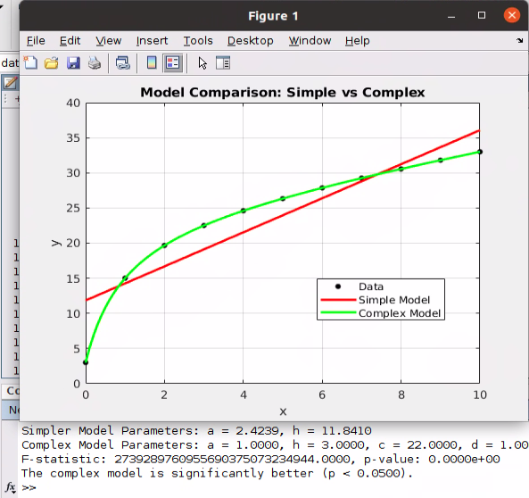
Once the algorithm has run through enough iterations, we can analyze the results. The code includes a simple visualization step that plots the estimated parameters, comparing them to the true values that were used to generate the synthetic data. This helps us understand how well the MCMC method has done in capturing the underlying structure of the data.

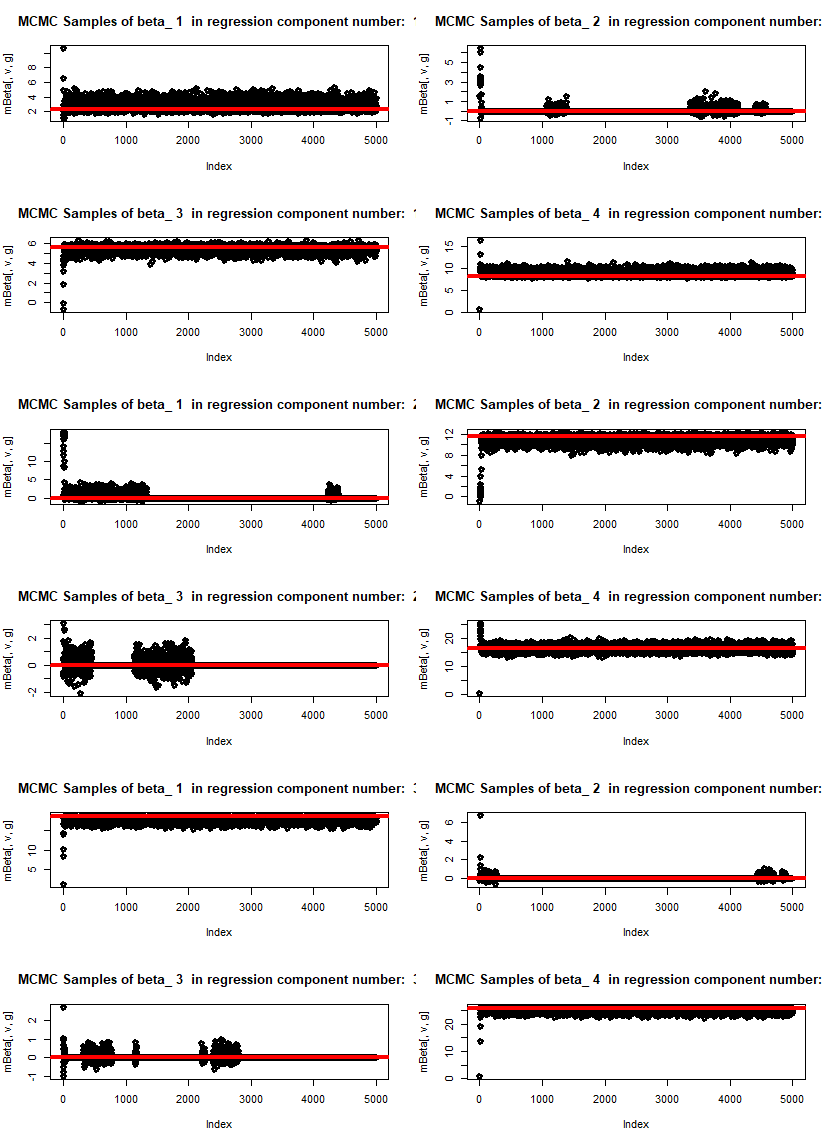
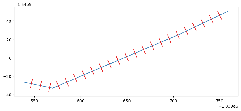
The graphs below present the outcome of the code with 5000 MCMC draws. We work with a mixture of three components, each with four potential explanatory variables. At the starting point we switch off some of the variables within individual mixtures. The algorithm is able to find only those features which have predictive power for the predicted variable. We plot the draws of individual beta parameters for all the components of regression. Some of them oscillate around 0. The red curve presents the true value of parameter beta in the data used for generating the mixture.

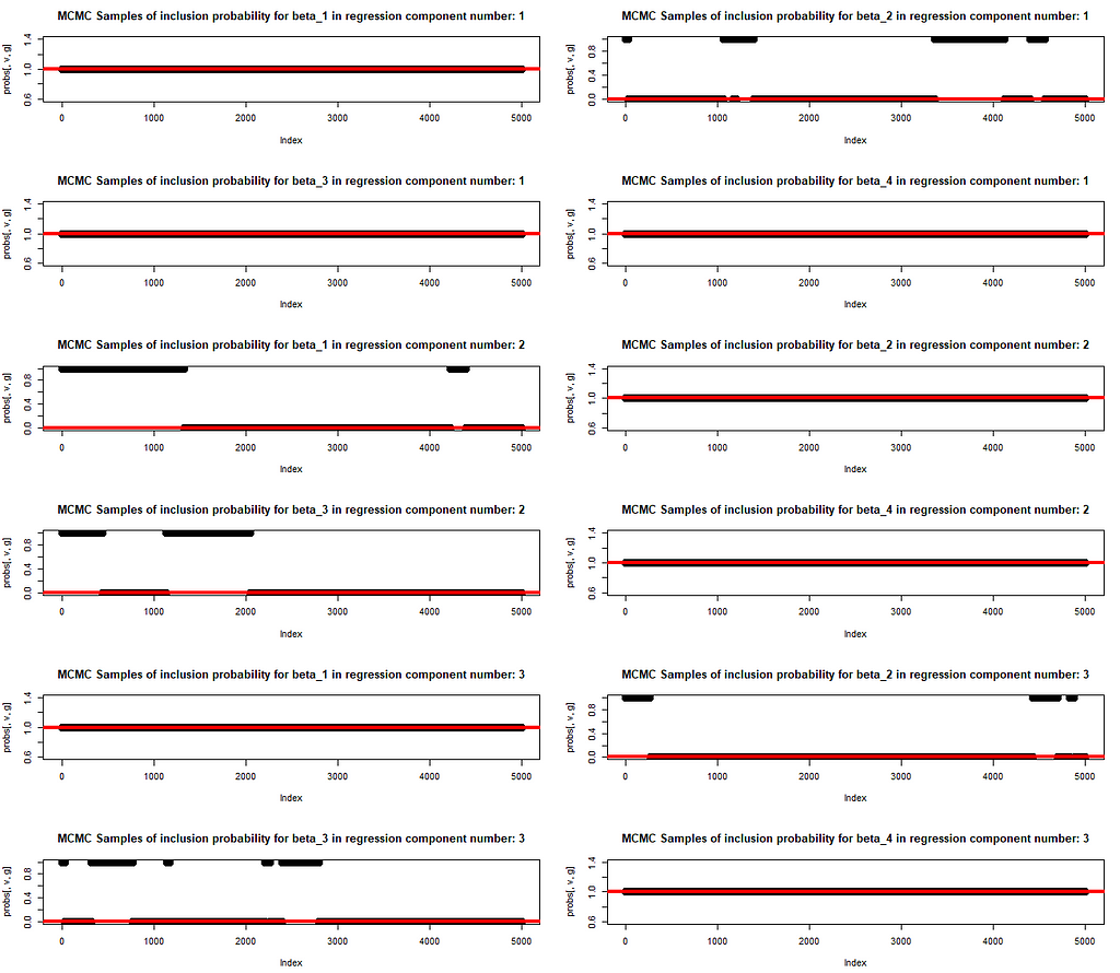
We also plot the MCMC draws of the inclusion probability. The red line at either 0 or 1 indicates if that parameter has been included in the original mixture of regression for generating the data. The learning of inclusion probability happens in parallel to the parameter training. This is exactly what allows for a trust in the trained values of betas. The model structure is revealed (i.e. the subset of variables with explanatory power is identified) and, at the same time, the correct values of beta are learnt.

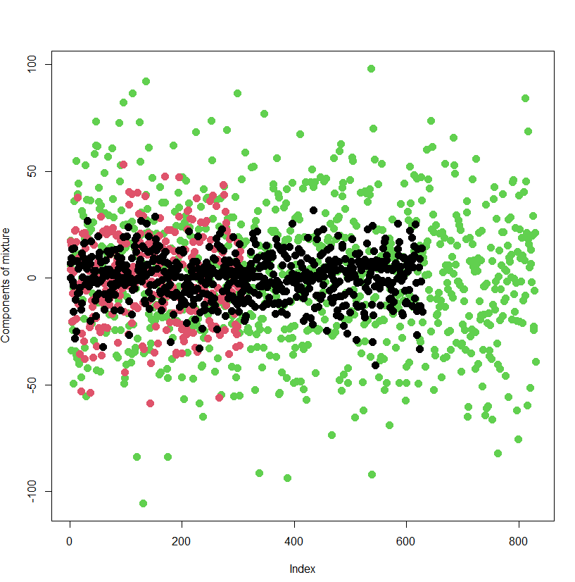
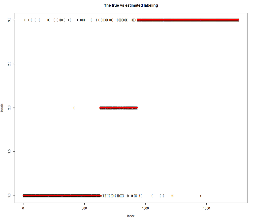
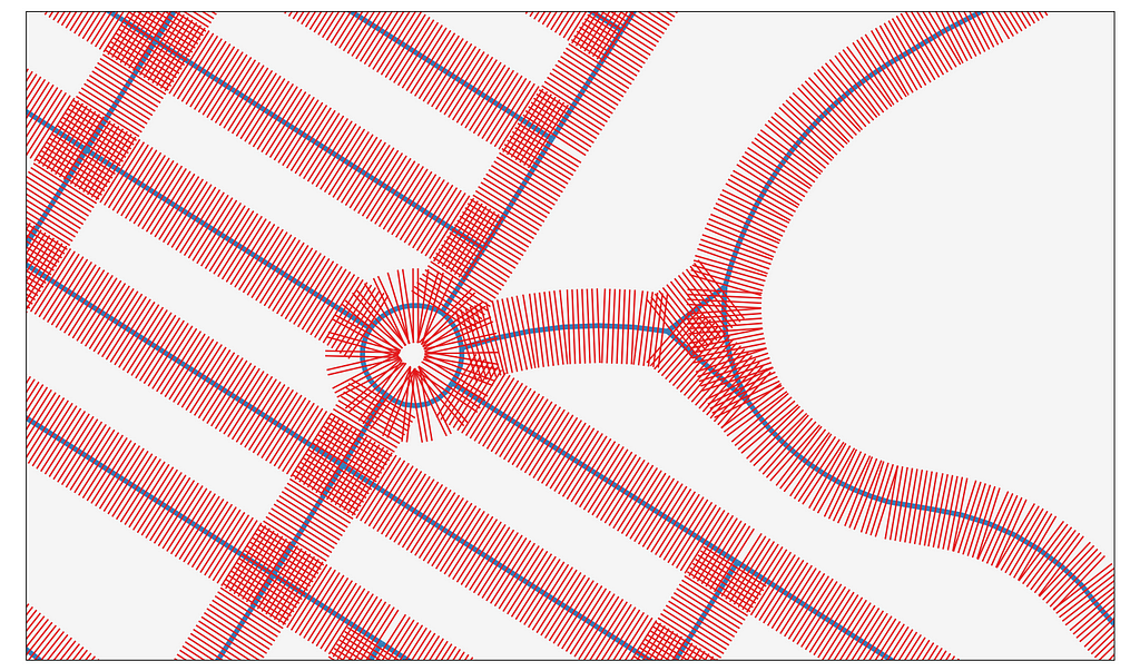
Finally, we present the outcome of classification of individual data points to the respective components of the mixture. The ability of the model to classify the data points to the component of the mixture they really stem from is great. The model has been wrong only in 6 % of cases.

Why This Is Interesting: The Power of Mixture Models in Action

What makes this approach particularly interesting is its ability to uncover hidden structures in data. Think about datasets that come from multiple sources or have inherent subpopulations, such as customer data, clinical trials, or even environmental measurements. Mixture models allow us to classify observations into these subpopulations without having to know their exact nature beforehand. The use of MCMC makes this even more powerful by allowing us to estimate parameters with high precision, even in cases where traditional estimation methods might fail.

Key Takeaways: Why MCMC and Mixture Models Matter

Mixture models with MCMC are incredibly powerful tools for analyzing complex datasets. By applying MCMC methods, we’re able to estimate parameters in situations where traditional models may struggle. This flexibility makes MCMC a go-to choice for many advanced data analysis tasks, from identifying customer segments to analyzing medical data or even predicting future trends based on historical patterns.

The code we explored in this article is just one example of how mixture models and MCMC can be applied in R. With some customization, you can apply these techniques to a wide variety of datasets, helping you uncover hidden insights and make more informed decisions.

For anyone interested in statistical modeling, machine learning, or data science, mastering mixture models and MCMC is a game-changer. These methods are versatile, powerful, and — when applied correctly — can unlock a wealth of insights from your data.

Final Thoughts

As data becomes increasingly complex, having the tools to model and interpret it effectively is more important than ever. Mixture models combined with MCMC offer a robust framework for handling multi-group data, and learning how to implement these techniques will significantly improve your analytical capabilities.

In the world of data science, mastering these advanced techniques opens up a vast array of possibilities, from business analytics to scientific research. With the R code provided, you now have a solid starting point for exploring mixture models and MCMC in your own projects, whether you’re uncovering hidden patterns in data or fine-tuning a predictive model. The next time you encounter a complex dataset, you’ll be well-equipped to dive deep and extract meaningful insights.

There is one important by product of the below implementation. Linear regression, while foundational in machine learning, often falls short in real-world applications due to its assumptions and limitations. One major issue is its assumption of a linear relationship between input features and the target variable, which rarely holds true in complex datasets.

Additionally, linear regression is sensitive to outliers and multicollinearity, where highly correlated features distort the model’s predictions. It also struggles with non-linear relationships and interactions between features, making it less flexible in capturing the complexity of modern data. In practice, data scientists often turn to more robust methods such as decision trees, random forests, support vector machines, and neural networks. These techniques can handle non-linearity, interactions, and large datasets more effectively, offering better predictive performance and adaptability in dynamic environments.

However, while above mentioned methods offer improved predictive power, they often come at the cost of interpretability. These models operate as “black boxes,” making it difficult to understand how input features are being transformed into predictions, which poses challenges for explain-ability and trust in critical decision-making applications.

So, is it possible to restore the shine of linear regression and make it a powerful tool again? Definitely, if you follow below implemented approach with the mixture of normal regression, you will feel the power of the underlying concept of linear regression with its great interpretability aspect!

Unless otherwise noted, all images are by the author.

---

Integrating Feature Selection into the Model Estimation was originally published in Towards Data Science on Medium, where people are continuing the conversation by highlighting and responding to this story.

Making the bears play nice

The Problem:

I needed to generate a transect every 10 feet across every street in New York City, and I had to do it in a New York Minute. The Generate Transects Along Lines tool built into ArcGIS Pro was going to take multiple days to run, so I had to come up with something at least slightly faster.

To solve this problem, I turned to two of my favorite bears, Geopandas and Polars, to use spatial algorithms and a dash of linear algebra to make 4.2 million transects in around 60 seconds.

Why Transects? In this circumstance, I would go on to use these transects to split up roadway lines into equal intervals for storm damage analysis. It is easier to split a line with another line than it is to split a line with a point, since you can guarantee they will intersect and you don’t have to worry about floating point imprecision. But, transects are super-useful for lots of application, such as sampling river depth profiles and creating a regular grid from a curvilinear line.

The Process:

First, I generated points along each line at 10 ft intervals using Geopandas built-in interpolate function. Once I had those points, I swapped them over to Polars, where I was able to take advantage of Polars’ built-in parallelism and intuitive syntax to quickly convert those points into (roughly) perpendicular transects. Finally, I put the transects into a GeoDataFrame for further spatial fun.

It may sound annoying to go back and forth between Geopandas and Polars, but each has its own advantages — GeoPandas has spatial operations, and Polars is wicked fast and I strongly prefer the syntax. The Polars .to_pandas() and .from_pandas() methods work so well that I barely notice the switch. While putting a panda bear and a polar bear into the same zoo enclosure may have disasterous consequences, in this circumstance they are able to play together quite nicely.

Requirements: This code was developed in a mamba environment with the following packages and has not been tested with other versions

geopandas==1.0.1
pandas==2.2.3
polars==1.18.0
Shapely==2.0.6

The data used in this article comes from NYC Open Data, and is available for download here. In this example, I am using the December 24, 2024 release of the NYC Street Centerlines.

Step 1: Generate points along lines every 10 feet with Geopandas

In order to create transects along each line, we first need to find the centerpoint of each transect. Since we want a transect every 10 ft, we will grab a point every 10 ft along every linestring in the dataset. We are also grab an additional point slightly offset from each transect point; this will allow us to findthe orientation needed to make the transect perpendicular to the original line. Before we get to all that, we need to load the data.

import geopandas as gpd

ROADS_LOC = r"NYC Street CenterlineNYC_Roads.shp"
ROADS_GDF = (
   gpd.read_file(ROADS_LOC)
      .reset_index(names="unique_id")
      .to_crs("epsg:6539")
)

In addition to loading the data, we also assign a unique_id to each road based on its index, and ensure the GeoDataFrame is in a projected coordinate system with feet as its base unit — since these road lines are in New York City, we use New York — Long Island State Plane as the coordinate reference system. The unique_id column will allow us to link our generated transects back to the original road segment.

Once the data has been loaded, we need to sample along every line at 10 ft intervals. We can accomplish this using the GeoPandas interpolate function, as below:

import pandas as pd
from typing import Tuple, Union


def interpolate_points(
    gdf: gpd.GeoDataFrame, distance: Union[float, int], is_transect: bool
) -> Tuple[gpd.GeoDataFrame, gpd.GeoDataFrame]:
    gdf = gdf.loc[gdf.length > distance]

    new_points = gdf.interpolate(distance)

    new_gdf = gpd.GeoDataFrame(
        geometry=new_points,
        data={
            "unique_id": gdf["unique_id"],
            "distance": distance,
            "is_transect": is_transect,
        },
        crs=gdf.crs,
    )

    return gdf, new_gdf

def get_road_points(roads: gpd.GeoDataFrame, segment_length: int) 
-> gpd.GeoDataFrame:
    working_roads = roads.copy()
    road_points = []
    for segment_distance in range(
        segment_length, int(roads.length.max()) + 1, segment_length
    ):
        working_roads, new_gdf = interpolate_points(
            working_roads, segment_distance - 1, False
        )
        road_points.append(new_gdf)
        
        working_roads, new_gdf = interpolate_points(
            working_roads, segment_distance, True
        )
        road_points.append(new_gdf)

    return pd.concat(road_points, ignore_index=True)

The function get_road_points() loops through all the segment distances in the roads GeoDataFrame, given a segment length s. Every iteration i, we select only roads which are longer than s * i. We sample a point along each line at s * i distance. These points will be the centerpoints of our new transects. Since we want to orient our new transects perpendicular to the line from which they spawned, we also sample a point at distance (s * i) -1. This gives us the approximate orientation of the line, which we will use later on when constructing the transects. As this method outputs a GeoSeries, we build a new GeoDataFrame, keeping the distance of the point along the line, whether the point will be used as a transect, and our previously created unique_id column. Finally, we concatenate all these GeoDataframes together, giving us something that looks like this:

Lets try it out with our roads dataset and see if it works:

import matplotlib.pyplot as plt

points_10ft = get_road_points(ROADS_GDF, 10)
fig, ax = plt.subplots(figsize=(10, 12))

ROADS_GDF.loc[ROADS_GDF['unique_id'] == 100].plot(ax=ax, color='blue')
points_10ft.loc[(points_10ft['unique_id'] == 100) & 
                (points_10ft['is_transect'])].plot(ax=ax, color='red')

Step 2: Use Polars and rotation matrices to turn those points into transects

Now that we have the points we need, we can use Polar’s from_pandas() function to convert our GeoDataFrame to Polars. Before we do that, we want to save the information from the geometry column — our x and y locations — and drop the geometry column.

import polars as pl 

def roads_to_polars(road_points: gpd.GeoDataFrame) -> pl.DataFrame:
    road_points.loc[:, "x"] = road_points.geometry.x
    road_points.loc[:, "y"] = road_points.geometry.y
    pl_points = pl.from_pandas(road_points.drop("geometry", axis=1))
    return pl_points

Finally, we have everything we need to construct our transects. In essence, all we have to do is find the angle of each transect, construct a transect of the requested length, and rotate and translate the transect so it is properly positioned in space. That may sound like a doozy, but if we break it down into steps we are not doing anything overly complicated.

1. Align each transect point with the point prior to it. This will allow us to orient each transect perpendicular to the original line by pivoting around the prior point. In fact, lets call the prior point the ‘pivot point’ to make this more clear.
2. Translate the transect point/pivot point pair so that the pivot point is at 0, 0. By doing this, we can easily rotate the transect point so that it sits at y = 0.
3. Rotate the transect point so that it sits at y = 0. By doing this, the math to construct new points which will form our transect becomes simple addition.
4. Construct new points above and below the rotated transect point so that we have a new line with distance equal to line length.
5. Rotate the new points back to the original orientation relative to the pivot point.
6. Translate the new points so that the pivot point returns to its original position.

Lets take a look at the code to do this. On my old laptop this code takes about 3 seconds to generate 4.2 million transects.

def make_lines(
  pl_points: pl.DataFrame, line_length: Union[float, int]) 
  -> pl.DataFrame:
    return (
        pl_points.sort("unique_id", "distance")
        # Pair each transect point with its preceding pivot point
        # over() groups by unique id, and shift(1) moves 
        # each column down by 1 row
        .with_columns(
            origin_x=pl.col("x").shift(1).over(pl.col("unique_id")),
            origin_y=pl.col("y").shift(1).over(pl.col("unique_id")),
        )
        # Remove pivot point rows
        .filter(pl.col("is_transect"))
        # Translate each point so the pivot is now (0, 0)
        .with_columns(
            translated_x=pl.col("x") - pl.col("origin_x"),
            translated_y=pl.col("y") - pl.col("origin_y"),
        )
        # Calculate angle theta between translated transect point and x-axis
        .with_columns(theta=pl.arctan2(
            pl.col("translated_y"), pl.col("translated_x")
            )
        )
        # Calculate terms in rotation matrix
        .with_columns(
          theta_cos=pl.col("theta").cos(), 
          theta_sin=pl.col("theta").sin()
        )
        # Add y-coordinates above and below x axis so we have a line of desired
        # length. Since we know that x = 1 (the distance between the transect
        # and pivot points), we don't have to explicitly set that term.
        .with_columns(
            new_y1=-line_length / 2,
            new_y2=line_length / 2,
        )
        # Apply rotation matrix to points (1, new_y1) and (1, new_y2) 
        # and translate back to the original location
        .with_columns(
            new_x1=pl.col("theta_cos")
            - (pl.col("new_y1") * pl.col("theta_sin"))
            + pl.col("origin_x"),
            new_y1=pl.col("theta_sin")
            + (pl.col("new_y1") * pl.col("theta_cos"))
            + pl.col("origin_y"),
            new_x2=pl.col("theta_cos")
            - (pl.col("new_y2") * pl.col("theta_sin"))
            + pl.col("origin_x"),
            new_y2=pl.col("theta_sin")
            + (pl.col("new_y2") * pl.col("theta_cos"))
            + pl.col("origin_y"),
        )
        # Construct a Well-Known Text representation of the transects
        # for easy conversion to GeoPandas
        .with_columns(
            wkt=pl.concat_str(
                pl.lit("LINESTRING ("),
                pl.col("new_x1"),
                pl.col("new_y1"),
                pl.lit(","),
                pl.col("new_x2"),
                pl.col("new_y2"),
                pl.lit(")"),
                separator=" ",
            )
        )
    )

How are we actually accomplishing the rotation?

We rotate the transect point about the origin using a rotation matrix. This is a 2×2 matrix which, when applied to a point in a 2d-plane, rotates the point θ degrees around the origin (0, 0).

To use it, all we need to do is calculate θ, then multiply the point (x, y) and the rotation matrix. This gives us the formula new_x = x*cos(θ)-y*sin(θ), new_y = x*sin(θ) + y*cos(θ). We calculate the result using this code:

.with_columns(
      new_x1=pl.col("theta_cos")
      - (pl.col("new_y1") * pl.col("theta_sin"))
      + pl.col("origin_x"),
      new_y1=pl.col("theta_sin")
      + (pl.col("new_y1") * pl.col("theta_cos"))
      + pl.col("origin_y"),
      new_x2=pl.col("theta_cos")
      - (pl.col("new_y2") * pl.col("theta_sin"))
      + pl.col("origin_x"),
      new_y2=pl.col("theta_sin")
      + (pl.col("new_y2") * pl.col("theta_cos"))
      + pl.col("origin_y"),
  )

We are able to simplify the calculation, since we know that x is always 1 for our points (x, y). Instead of calculating x*cos(θ)-y*sin(θ) to find the x value of a rotated point, we can just do cos(θ)-y*sin(θ), saving us a little bit of computation. Of course, this won’t work if your pivot point and transect point are not 1 unit apart, but for our purposes it is just fine. Once we have the rotation completed, all we have to do is translate the newly rotated points by the distance between the pivot point and (0,0), and boom, we are done. If you are interested in learning more about linear algebra and affine transformations, I highly reccomend the 3Blue1Brown series Essence of Linear Algebra.

Using the above functions, we can take our GeoDataFrame, convert it to Polars, and calculate new transects like so:

points_10ft_pl = roads_to_polars(points_10ft)
transects_10ft = make_lines(points_10ft_pl, 10)
transects_10ft.select(['unique_id', 'wkt'])

Step 3: Convert the transects back to Geopandas

Finally! We have the geometric coordinates of the transects we need, but we want them in a GeoDataFrame so we can go back to the comfort of GIS operations. Since we constructed our new transects as WKT Linestrings at the end of the make_lines() function, the code to do so is simple:

transects_gdf = gpd.GeoDataFrame(
    crs=ROADS_GDF.crs,
    data={"unique_id": transects_10ft.select("unique_id").to_series()},
    geometry=gpd.GeoSeries.from_wkt(
        transects_10ft.select("wkt").to_series().to_list()
    ),
)

And thats it! We now have a GeoDataFrame with 4.2 million transects, each linked to their original roadway using the unique_id column.

Lets check out our new geometry:

ROAD_ID = 98237
fig, ax = plt.subplots(figsize=(10, 12))
ROADS_GDF.loc[ROADS_GDF['unique_id'] == ROAD_ID].plot(ax=ax, color='blue')
transects_gdf.loc[transects_gdf['unique_id'] == ROAD_ID].plot(ax=ax, color='green')
ax.set_aspect("equal")

Transects spaced 10ft apart along a pedestrian pathLooks good! We are losing a little bit of precision with the WKT conversion, so there is probably a better way to do that, but it works well enough for me.

Putting it all Together

For your convenience, I have combined the code to generate the transects below. This will only work with data projected to a planar coordinate system, and if you want to use a pivot point that is further than 1 unit from a transect point, you will need to modify the code.

from typing import Tuple, Union

import geopandas as gpd
import pandas as pd
import polars as pl


def interpolate_points(
    gdf: gpd.GeoDataFrame, distance: Union[float, int], is_transect: bool
) -> Tuple[gpd.GeoDataFrame, gpd.GeoDataFrame]:
    gdf = gdf.loc[gdf.length > distance]

    new_points = gdf.interpolate(distance)

    new_gdf = gpd.GeoDataFrame(
        geometry=new_points,
        data={
            "unique_id": gdf["unique_id"],
            "distance": distance,
            "is_transect": is_transect,
        },
        crs=gdf.crs,
    )

    return gdf, new_gdf


def get_road_points(roads: gpd.GeoDataFrame, segment_length: int) -> gpd.GeoDataFrame:
    working_roads = roads.copy()
    road_points = []
    for segment_distance in range(
        segment_length, int(roads.length.max()) + 1, segment_length
    ):
        working_roads, new_gdf = interpolate_points(
            working_roads, segment_distance - 1, False
        )
        road_points.append(new_gdf)
        
        working_roads, new_gdf = interpolate_points(
            working_roads, segment_distance, True
        )
        road_points.append(new_gdf)

    return pd.concat(road_points, ignore_index=True)


def roads_to_polars(road_points: gpd.GeoDataFrame) -> pl.DataFrame:
    road_points.loc[:, "x"] = road_points.geometry.x
    road_points.loc[:, "y"] = road_points.geometry.y
    pl_points = pl.from_pandas(road_points.drop("geometry", axis=1))
    return pl_points


def make_lines(pl_points: pl.DataFrame, line_length: Union[float, int]) -> pl.DataFrame:
    return (
        pl_points.sort("unique_id", "distance")
        .with_columns(
            origin_x=pl.col("x").shift(1).over(pl.col("unique_id")),
            origin_y=pl.col("y").shift(1).over(pl.col("unique_id")),
        )
        .filter(pl.col("is_transect"))
        .with_columns(
            translated_x=pl.col("x") - pl.col("origin_x"),
            translated_y=pl.col("y") - pl.col("origin_y"),
        )
        .with_columns(theta=pl.arctan2(pl.col("translated_y"), pl.col("translated_x")))
        .with_columns(theta_cos=pl.col("theta").cos(), theta_sin=pl.col("theta").sin())
        .with_columns(
            new_y1=-line_length / 2,
            new_y2=line_length / 2,
        )
        .with_columns(
            new_x1=pl.col("theta_cos")
            - (pl.col("new_y1") * pl.col("theta_sin"))
            + pl.col("origin_x"),
            new_y1=pl.col("theta_sin")
            + (pl.col("new_y1") * pl.col("theta_cos"))
            + pl.col("origin_y"),
            new_x2=pl.col("theta_cos")
            - (pl.col("new_y2") * pl.col("theta_sin"))
            + pl.col("origin_x"),
            new_y2=pl.col("theta_sin")
            + (pl.col("new_y2") * pl.col("theta_cos"))
            + pl.col("origin_y"),
        )
        .with_columns(
            wkt=pl.concat_str(
                pl.lit("LINESTRING ("),
                pl.col("new_x1"),
                pl.col("new_y1"),
                pl.lit(","),
                pl.col("new_x2"),
                pl.col("new_y2"),
                pl.lit(")"),
                separator=" ",
            )
        )
    )

ROADS_LOC = r"NYC Street CenterlineNYC_Roads.shp"
ROADS_GDF = gpd.read_file(ROADS_LOC).reset_index(names="unique_id").to_crs("epsg:6539")

points_10ft = get_road_points(roads=ROADS_GDF, segment_length=10)
points_10ft_pl = roads_to_polars(road_points=points_10ft)
transects_10ft = make_lines(pl_points=points_10ft_pl, line_length=10)
transects_gdf = gpd.GeoDataFrame(
    crs=ROADS_GDF.crs,
    data={"unique_id": transects_10ft.select("unique_id").to_series()},
    geometry=gpd.GeoSeries.from_wkt(transects_10ft.select("wkt").to_series().to_list()),
)

Thanks for reading! There are probably a lot more ways this code could be optimized or made more flexible, but it solved a huge problem for me and cut down compute time from days to seconds. With a little bit of theory and knowing when to use what tool, problems that previously seem insurmountable become shockingly easy. It only took me about 30 minutes and a little wikipedia linear algebra referesher to write the code for this post, saving me tons of time and, more importantly, protecting me from having to explain to a client why a project was pointlessly delayed. Let me know if this was helpful to you!

Unless otherwise noted, all images are by the author.

---

Harnessing Polars and Geopandas to Generate Millions of Transects in Seconds was originally published in Towards Data Science on Medium, where people are continuing the conversation by highlighting and responding to this story.